Χωροθέτηση Επιχείρησης Η σημασία της χωροθέτησης Η χωροθέτηση μιας επιχείρησης έχει μεσο- μακροπρόθεσμα καταλυτική επιρροή στο κόστος λειτουργίας, στην.

Παρουσίαση με θέμα: "Χωροθέτηση Επιχείρησης Η σημασία της χωροθέτησης Η χωροθέτηση μιας επιχείρησης έχει μεσο- μακροπρόθεσμα καταλυτική επιρροή στο κόστος λειτουργίας, στην."— Μεταγράφημα παρουσίασης:

1

2 Χωροθέτηση Επιχείρησης

3 Η σημασία της χωροθέτησης Η χωροθέτηση μιας επιχείρησης έχει μεσο- μακροπρόθεσμα καταλυτική επιρροή στο κόστος λειτουργίας, στην τιμολογιακή πολιτική και στην γενικότερη ανταγωνιστικότητα της επιχείρησης. Εξαγωγές: 1962 – 12% παγκόσμιου GNP 1995 – 30% παγκόσμιου GNP

4 Σύγχρονες Τάσεις Γεωγραφική διασπορά Βελτιωμένες μεταφορές Μείωση εμποδίων στο διεθνές εμπόριο Υποβάθμιση αστικών περιοχών Διεθνοποίηση παραγωγής Αναπτυσσόμενες αγορές Διαφοροποιήσεις κόστους εργασίας

5 N.A. Ασία Taiwan - εξάγει 70% της παραγωγής της - παράγει 20% των PCs παγκοσμίως Japan South Korea Taiwan Singapore Hong Kong China Μέγιστος ρυθμός ανάπτυξης εμπορίου

6 Β. Αμερική Mexico (1996): 2,000 νέα εργοστάσια 500,000 εργαζόμενοι Φθηνό εργατικό κόστος, χαμηλή παραγωγικότητα, ελλειμματικές υποδομές. USΑ: > 3,000 νέες χωροθετήσεις / χρόνο > 7,500 επεκτάσεις / χρόνο NAFTA (North American Free Trade Agreement) Canada-Mexico-United States

7 Ευρωπαϊκή Ένωση European Union (EU) των 15 μελών…

8 European Union (EU) των 10 νέων μελών + … Ζωτικός χώρος 410 εκατομμυρίων πολιτών Russia Ευρωπαϊκή Ένωση

9 Διαχείριση σε παγκόσμια κλίμακα Επικοινωνία σε ξένες γλώσσες Διαφορετικά πρότυπα και έθιμα Διαχείριση ανθρώπινου δυναμικού Άγνωστη νομοθεσία και κανονιστικό πλαίσιο Απρόβλεπτα κόστη

10 Αποφασίζοντας για μια νέα επιχειρηματική μονάδα  Μεταβολή στη ζήτηση (θετική ή αρνητική).  Νέο προϊόν.  Αλλαγές στο οικονομικό περιβάλλον, π.χ. εργατικό κόστος, κόστος πρώτων υλών, πηγές πρώτων υλών, υποστηρικτικές επιχειρήσεις.  Κυβερνητικές ρυθμίσεις, π.χ. φορολογικοί νόμοι, αναπτυξιακά κίνητρα, περιβαλλοντικές ρυθμίσεις.

11 Ανταγωνιστικά Κριτήρια χωροθέτησης επιχειρήσεων Ανάγκη παραγωγής κοντά στην αγορά (ταχύτητα απόκρισης, διασυνοριακό εμπόριο, μεταφορικά κόστη) Ανάγκη παραγωγής κοντά στο κατάλληλο στελεχιακό δυναμικό (χαμηλό κόστος εργασίας, υψηλό επίπεδο εκπαίδευσης, επιχειρησιακή κουλτούρα)

12 Βασικά στάδια στην απόφαση για νέα χωροθέτηση 1. Συστηματική ανάλυση της ανάγκης για νέα χωροθέτηση. 2. Αναγνώριση των κρίσιμων παραγόντων για τον προσδιορισμό της θέσης. 3. Επιλογή γενικής γεωγραφικής θέσης. 4. Συγκεκριμένη επιλογή θέσης επιχείρησης.

13 Σ1: Ανάλυση της ανάγκης για νέα χωροθέτηση Μέγεθος Μονάδας Κόστος Κόστος Παραγωγής Κόστος Μεταφοράς Συνολικό Κόστος Ιδανικό Μέγεθος

14 Σ2: Κρίσιμοι παράγοντες προσδιορισμού θέσης Πρόσβαση στις αγορές και στους προμηθευτές Απόσταση από την κεντρική επιχείρηση Θέση ανταγωνιστών Κόστη παραγωγής και μεταφορών Αναπτυξιακά κίνητρα Περιβαλλοντικοί όροι Πρόσβαση στην τεχνολογία Εργασιακό κλίμα Ποιότητα ζωής Πολιτική σταθερότητα

15 - Κρίσιμοι Παράγοντες - Βιομηχανία  Απόσταση από την κεντρική επιχείρηση  Φορολογία, υποδομές, κόστος γής  Πρόσβαση στους προμηθευτές  Ευνοϊκό εργασιακό κλίμα  Πρόσβαση στις αγορές  Ποιότητα ζωής

16 - Κρίσιμοι Παράγοντες - Υπηρεσίες  Πρόσβαση στους πελάτες  Κόστος μεταφοράς  Θέση ανταγωνισμού  Site-specific Factors

17 Χωροθέτηση ανεξάρτητης μεμονωμένης μονάδας Επέκταση υπάρχουσας μονάδας Κατασκευή νέας μονάδας Μεταφορά μονάδας σε νέα θέση

18 Επέκταση υπάρχουσας μονάδας +Ενιαίο διοικητικό σχήμα +Μειωμένο κόστος κατασκευής +Μικρός χρόνος κατασκευής –Μικρότερη ευελιξία –Δυσκολότερη διαχείριση υλικών –Περισσότερο σύνθετη παραγωγή –Έλλειψη χώρου

19 Κατασκευή νέας μονάδας +Μικρότερος κίνδυνος απώλειας παραγωγής +Αποφυγή εργασιακών προβλημάτων +Εκσυγχρονισμός με νέα μηχανήματα +Μειωμένα μεταφορικά κόστη –Κόστος επένδυσης

20 Σ3: Επιλογή γενικής γεωγραφικής θέσης 1.Επιλογή παραγόντων απόφασης. 2.Διαμόρφωση λίστας εναλλακτικών περιοχών. 3.Συλλογή στατιστικών δεδομένων. 4.Συγκριτική ανάλυση με ενιαίο ποσοτικό δείκτη. 5.Εξειδίκευση ποσοτικού δείκτη.

21 Εργαλεία ανάλυσης Αξιολόγηση προτεραιοτήτων Μοντέλο Μεταφορών –Μέση απόσταση –Ζυγισμένη Απόσταση –Κέντρο Βάρους Ανάλυση σημείου ισορροπίας

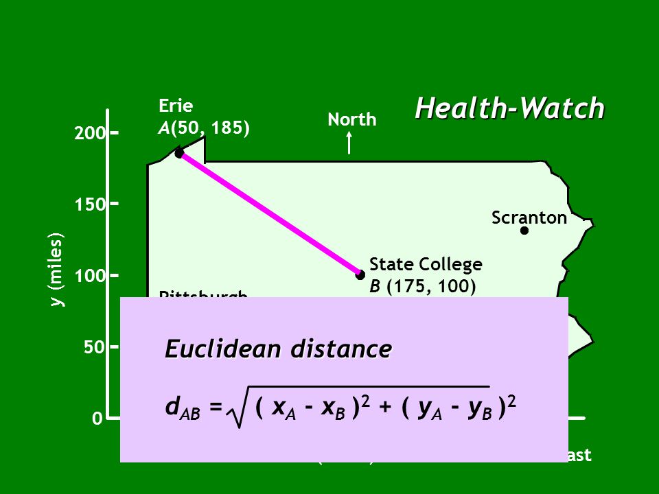
22 Παράδειγμα Health-Watch North

23 Health-Watch ΠαράγονταςΕιδικό ΒάροςΒαθμός Σύνολο ασθενομιλίων ανά χρόνο254 Χρήση μονάδας203 Μέσος χρόνος μεταφοράς επείγοντος203 Πρόσβαση σε αυτοκινητόδρομο154 Κόστος γης και κατασκευής101 Προτίμηση εργαζομένων105

24 Health-Watch North Location Factor WeightScore Total Patient miles per month254 Facility utilization203 Average time per emergency trip203 Expressway accessibility154 Land and construction costs101 Employee preference105 Weighted Score

25 Health-Watch North Location Factor WeightScore Total Patient miles per month254 Facility utilization203 Average time per emergency trip203 Expressway accessibility154 Land and construction costs101 Employee preference105 WS=(25 x 4) Weighted Score

26 Health-Watch North Location Factor WeightScore Total Patient miles per month254 Facility utilization203 Average time per emergency trip203 Expressway accessibility154 Land and construction costs101 Employee preference105 WS=(25 x 4) + (20 x 3) Weighted Score

27 Health-Watch North Location FactorWeightScore Total Patient miles per month254 Facility utilization203 Average time per emergency trip203 Expressway accessibility154 Land and construction costs101 Employee preference105 WS=(25 x 4) + (20 x 3) + (20 x 3) Weighted Score

28 Health-Watch North Location FactorWeightScore Total Patient miles per month254 Facility utilization203 Average time per emergency trip203 Expressway accessibility154 Land and construction costs101 Employee preference105 WS=(25 x 4) + (20 x 3) + (20 x 3) + (15 x4) + (10 x 1) + (10 x 5) Weighted Score

29 Health-Watch North Location FactorWeightScore Total Patient miles per month254 Facility utilization203 Average time per emergency trip203 Expressway accessibility154 Land and construction costs101 Employee preference105 WS=340 Weighted Score

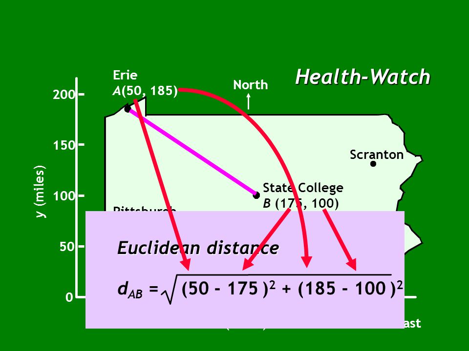
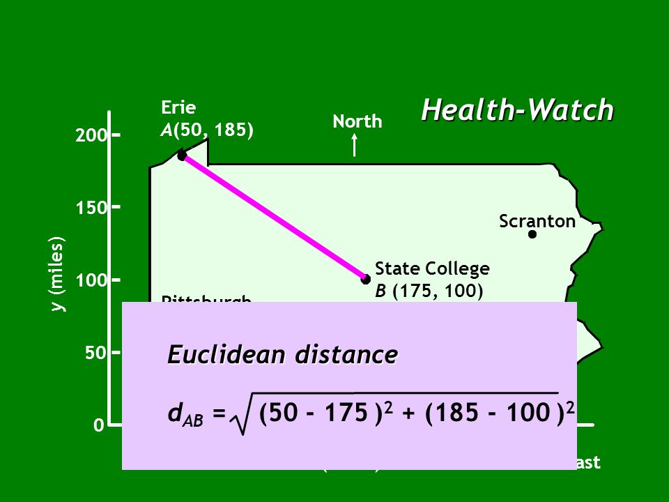
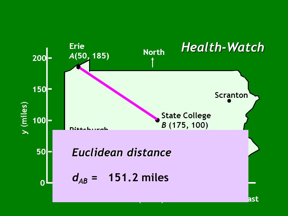
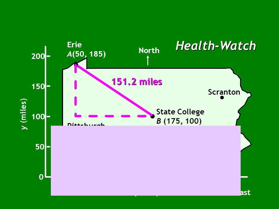
30 Health-Watch Erie A(50, 185) Pittsburgh Harrisburg Philadelphia Scranton Uniontown North 0 50 100 150 200 y (miles) x (miles) 50100150200250300 East State College B (175, 100)

31

32

33

34

35

36 Health-Watch Erie A(50, 185) Pittsburgh Harrisburg Philadelphia Scranton Uniontown North 0 50 100 150 200 y (miles) x (miles) 50100150200250300 East State College B (175, 100) 151.2 miles

37 Health-Watch Erie A(50, 185) Pittsburgh Harrisburg Philadelphia Scranton Uniontown North 0 50 100 150 200 y (miles) x (miles) 50100150200250300 East State College B (175, 100) 151.2 miles Rectilinear distance d AB = | x A - x B | + | y A - y B |

38 Health-Watch Erie A(50, 185) Pittsburgh Harrisburg Philadelphia Scranton Uniontown North 0 50 100 150 200 y (miles) x (miles) 50100150200250300 East State College B (175, 100) 151.2 miles Rectilinear distance d AB = | 50 - 175 | + | 185 - 100 |

39 Health-Watch Erie A(50, 185) Pittsburgh Harrisburg Philadelphia Scranton Uniontown North 0 50 100 150 200 y (miles) x (miles) 50100150200250300 East State College B (175, 100) 151.2 miles Rectilinear distance d AB = | 50 - 175 | + | 185 - 100 |

40 Health-Watch Erie A(50, 185) Pittsburgh Harrisburg Philadelphia Scranton Uniontown North 0 50 100 150 200 y (miles) x (miles) 50100150200250300 East State College B (175, 100) 151.2 miles Rectilinear distance d AB = 210 miles

41 Health-Watch Erie A(50, 185) Pittsburgh Harrisburg Philadelphia Scranton Uniontown North 0 50 100 150 200 y (miles) x (miles) 50100150200250300 East State College B (175, 100) 151.2 miles 210 miles

42 Figure 9.3 Health-Watch Erie A (50, 185) North Enter the x and y coordinates of the two towns. xy Erie (Point A)50185 State College (Point B)175100 To find the Euclidian distance, subtract the second town’s x value from that of the first town, and square the result. Do the same with the two y values. Then add the two and compute the square root. (Erie x – State College x) 2 15.625Euclidian distance151.16 (Erie y – State College y) 2 7,225 To find the rectilinear distance, get the absolute value of the result of subtracting the second town’s x from the first town’s. Do the same with y. Then add the absolute distances together. (Erie x – State College x)125Rectilinear distance210 (Erie y – State College y)85 Tutor 9.2 - Distance Measures

43 Health-Watch North B A C E G F D (2.5, 4.5) [2] (2.5, 2.5) [5] (5, 2) [7] (7, 2) [20] (9, 2.5) [14] (8, 5) [10] (5.5, 4.5) [10] x (miles) East 12345678910 1 2 3 4 5 6 0 y (miles)

44 Health-Watch (a) Locate at C (5.5, 4.5) North B A C E G F D (2.5, 4.5) [2] (2.5, 2.5) [5] (5, 2) [7] (7, 2) [20] (9, 2.5) [14] (8, 5) [10] (5.5, 4.5) [10] x (miles) East 12345678910 1 2 3 4 5 6 0 y (miles) Census PopulationDistance Tract(x,y)(l)(d)ld

45 Health-Watch (a) Locate at C (5.5, 4.5) North B A C E G F D (2.5, 4.5) [2] (2.5, 2.5) [5] (5, 2) [7] (7, 2) [20] (9, 2.5) [14] (8, 5) [10] (5.5, 4.5) [10] x (miles) East 12345678910 1 2 3 4 5 6 0 y (miles) Census PopulationDistance Tract(x,y)(l)(d)ld A(2.5, 4.5)2

46 Health-Watch (a) Locate at C (5.5, 4.5) North B A C E G F D (2.5, 4.5) [2] (2.5, 2.5) [5] (5, 2) [7] (7, 2) [20] (9, 2.5) [14] (8, 5) [10] (5.5, 4.5) [10] x (miles) East 12345678910 1 2 3 4 5 6 0 y (miles) Census PopulationDistance Tract(x,y)(l)(d)ld A(2.5, 4.5)2

47 Health-Watch (a) Locate at C (5.5, 4.5) North B A C E G F D (2.5, 4.5) [2] (2.5, 2.5) [5] (5, 2) [7] (7, 2) [20] (9, 2.5) [14] (8, 5) [10] (5.5, 4.5) [10] x (miles) East 12345678910 1 2 3 4 5 6 0 y (miles) Census PopulationDistance Tract(x,y)(l)(d)ld A(2.5, 4.5)2 5.5 - 2.5 = 3

48 Health-Watch (a) Locate at C (5.5, 4.5) North B A C E G F D (2.5, 4.5) [2] (2.5, 2.5) [5] (5, 2) [7] (7, 2) [20] (9, 2.5) [14] (8, 5) [10] (5.5, 4.5) [10] x (miles) East 12345678910 1 2 3 4 5 6 0 y (miles) Census PopulationDistance Tract(x,y)(l)(d)ld A(2.5, 4.5)2 5.5 - 2.5 = 3 4.5 - 4.5 = 0

49 Health-Watch (a) Locate at C (5.5, 4.5) North B A C E G F D (2.5, 4.5) [2] (2.5, 2.5) [5] (5, 2) [7] (7, 2) [20] (9, 2.5) [14] (8, 5) [10] (5.5, 4.5) [10] x (miles) East 12345678910 1 2 3 4 5 6 0 y (miles) Census PopulationDistance Tract(x,y)(l)(d)ld A(2.5, 4.5)23 + 0 = 3 5.5 - 2.5 = 3 4.5 - 4.5 = 0

50 Health-Watch (a) Locate at C (5.5, 4.5) North B A C E G F D (2.5, 4.5) [2] (2.5, 2.5) [5] (5, 2) [7] (7, 2) [20] (9, 2.5) [14] (8, 5) [10] (5.5, 4.5) [10] x (miles) East 12345678910 1 2 3 4 5 6 0 y (miles) Census PopulationDistance Tract(x,y)(l)(d)ld A(2.5, 4.5)23 + 0 = 36 2 * 3 = 6

51 Health-Watch (a) Locate at C (5.5, 4.5) North B A C E G F D (2.5, 4.5) [2] (2.5, 2.5) [5] (5, 2) [7] (7, 2) [20] (9, 2.5) [14] (8, 5) [10] (5.5, 4.5) [10] x (miles) East 12345678910 1 2 3 4 5 6 0 y (miles) Census PopulationDistance Tract(x,y)(l)(d)ld A(2.5, 4.5)23 + 0 = 36

52 Health-Watch (a) Locate at C (5.5, 4.5) North B A C E G F D (2.5, 4.5) [2] (2.5, 2.5) [5] (5, 2) [7] (7, 2) [20] (9, 2.5) [14] (8, 5) [10] (5.5, 4.5) [10] x (miles) East 12345678910 1 2 3 4 5 6 0 y (miles) Census PopulationDistance Tract(x,y)(l)(d)ld A(2.5, 4.5)23 + 0 = 36 E(8, 5)10

53 Health-Watch (a) Locate at C (5.5, 4.5) North B A C E G F D (2.5, 4.5) [2] (2.5, 2.5) [5] (5, 2) [7] (7, 2) [20] (9, 2.5) [14] (8, 5) [10] (5.5, 4.5) [10] x (miles) East 12345678910 1 2 3 4 5 6 0 y (miles) Census PopulationDistance Tract(x,y)(l)(d)ld A(2.5, 4.5)23 + 0 = 36 E(8, 5)10 2.5 + 0.5 = 3 8 - 5.5 = 2.5 5 - 4.5 = 0.5

54 Health-Watch (a) Locate at C (5.5, 4.5) North B A C E G F D (2.5, 4.5) [2] (2.5, 2.5) [5] (5, 2) [7] (7, 2) [20] (9, 2.5) [14] (8, 5) [10] (5.5, 4.5) [10] x (miles) East 12345678910 1 2 3 4 5 6 0 y (miles) Census PopulationDistance Tract(x,y)(l)(d)ld A(2.5, 4.5)23 + 0 = 36 E(8, 5)102.5 + 0.5 = 330 10 * 3 = 30

55 Health-Watch (a) Locate at C (5.5, 4.5) North B A C E G F D (2.5, 4.5) [2] (2.5, 2.5) [5] (5, 2) [7] (7, 2) [20] (9, 2.5) [14] (8, 5) [10] (5.5, 4.5) [10] x (miles) East 12345678910 1 2 3 4 5 6 0 y (miles) Census PopulationDistance Tract(x,y)(l)(d)ld A(2.5, 4.5)23 + 0 = 36 E(8, 5)102.5 + 0.5 = 330

56 Health-Watch (a) Locate at C (5.5, 4.5) North B A C E G F D (2.5, 4.5) [2] (2.5, 2.5) [5] (5, 2) [7] (7, 2) [20] (9, 2.5) [14] (8, 5) [10] (5.5, 4.5) [10] x (miles) East 12345678910 1 2 3 4 5 6 0 y (miles) Tractld A6 B25 C0 D21 E30 F80 G77 Total239

57 Health-Watch (b) Locate at F (7, 2) North B A C E G F D (2.5, 4.5) [2] (2.5, 2.5) [5] (5, 2) [7] (7, 2) [20] (9, 2.5) [14] (8, 5) [10] (5.5, 4.5) [10] x (miles) East 12345678910 1 2 3 4 5 6 0 y (miles)

58 Health-Watch (b) Locate at F (7, 2) North B A C E G F D (2.5, 4.5) [2] (2.5, 2.5) [5] (5, 2) [7] (7, 2) [20] (9, 2.5) [14] (8, 5) [10] (5.5, 4.5) [10] x (miles) East 12345678910 1 2 3 4 5 6 0 y (miles)

59 Health-Watch (b) Locate at F (7, 2) North B A C E G F D (2.5, 4.5) [2] (2.5, 2.5) [5] (5, 2) [7] (7, 2) [20] (9, 2.5) [14] (8, 5) [10] (5.5, 4.5) [10] x (miles) East 12345678910 1 2 3 4 5 6 0 y (miles) Tractld A14 B25 C40 D14 E40 F0 G35 Total168

60 Health-Watch Alternative Locations North x (miles) East 12345678910 1 2 3 4 5 6 0 y (miles)

61 Health-Watch Alternative Locations North x (miles) East 12345678910 1 2 3 4 5 6 0 y (miles) 391 355 331 326 283 247 223 233 197 173 253 233 228 168 218

62 Health-Watch Center of Gravity Approach North B A C E G F D (2.5, 4.5) [2] (2.5, 2.5) [5] (5, 2) [7] (7, 2) [20] (9, 2.5) [14] (8, 5) [10] (5.5, 4.5) [10] x (miles) East 12345678910 1 2 3 4 5 6 0 y (miles)

63 Health-Watch Center of Gravity Approach North B A C E G F D (2.5, 4.5) [2] (2.5, 2.5) [5] (5, 2) [7] (7, 2) [20] (9, 2.5) [14] (8, 5) [10] (5.5, 4.5) [10] x (miles) East 12345678910 1 2 3 4 5 6 0 y (miles) Census Population Tract(x,y)(l)lxly A(2.5, 4.5)2 B(2.5, 2.5)5 C(5.5, 4.5)10 D(5, 2)7 E(8, 5)10 F(7, 2)20 G(9, 2.5)14

64 Health-Watch Center of Gravity Approach North B A C E G F D (2.5, 4.5) [2] (2.5, 2.5) [5] (5, 2) [7] (7, 2) [20] (9, 2.5) [14] (8, 5) [10] (5.5, 4.5) [10] x (miles) East 12345678910 1 2 3 4 5 6 0 y (miles) Census Population Tract(x,y)(l)lxly A(2.5, 4.5)25 B(2.5, 2.5) C(5.5, 4.5) D(5, 2) E(8, 5) F(7, 2) G(9, 2.5)

65 Health-Watch Center of Gravity Approach North B A C E G F D (2.5, 4.5) [2] (2.5, 2.5) [5] (5, 2) [7] (7, 2) [20] (9, 2.5) [14] (8, 5) [10] (5.5, 4.5) [10] x (miles) East 12345678910 1 2 3 4 5 6 0 y (miles) Census Population Tract(x,y)(l)lxly A(2.5, 4.5)259 B(2.5, 2.5) C(5.5, 4.5) D(5, 2) E(8, 5) F(7, 2) G(9, 2.5)

66 Health-Watch Center of Gravity Approach North B A C E G F D (2.5, 4.5) [2] (2.5, 2.5) [5] (5, 2) [7] (7, 2) [20] (9, 2.5) [14] (8, 5) [10] (5.5, 4.5) [10] x (miles) East 12345678910 1 2 3 4 5 6 0 y (miles) Census Population Tract(x,y)(l)lxly A(2.5, 4.5)259 B(2.5, 2.5) C(5.5, 4.5) D(5, 2) E(8, 5) F(7, 2) G(9, 2.5)

67 Health-Watch Center of Gravity Approach North B A C E G F D (2.5, 4.5) [2] (2.5, 2.5) [5] (5, 2) [7] (7, 2) [20] (9, 2.5) [14] (8, 5) [10] (5.5, 4.5) [10] x (miles) East 12345678910 1 2 3 4 5 6 0 y (miles) Census Population Tract(x,y)(l)lxly A(2.5, 4.5)259 B(2.5, 2.5)512.512.5 C(5.5, 4.5)105545 D(5, 2)73514 E(8, 5)108050 F(7, 2)2014040 G(9, 2.5)1412635

68 Health-Watch Center of Gravity Approach North B A C E G F D (2.5, 4.5) [2] (2.5, 2.5) [5] (5, 2) [7] (7, 2) [20] (9, 2.5) [14] (8, 5) [10] (5.5, 4.5) [10] x (miles) East 12345678910 1 2 3 4 5 6 0 y (miles) Census Population Tract(x,y)(l)lxly A(2.5, 4.5)259 B(2.5, 2.5)512.512.5 C(5.5, 4.5)105545 D(5, 2)73514 E(8, 5)108050 F(7, 2)2014040 G(9, 2.5)1412635 Totals68453.5205.5 Totals68453.5205.5

69 Health-Watch Center of Gravity Approach North B A C E G F D (2.5, 4.5) [2] (2.5, 2.5) [5] (5, 2) [7] (7, 2) [20] (9, 2.5) [14] (8, 5) [10] (5.5, 4.5) [10] x (miles) East 12345678910 1 2 3 4 5 6 0 y (miles) Census Population Tract(x,y)(l)lxly A(2.5, 4.5)259 B(2.5, 2.5)512.512.5 C(5.5, 4.5)105545 D(5, 2)73514 E(8, 5)108050 F(7, 2)2014040 G(9, 2.5)1412635 Totals68453.5205.5 Totals68453.5205.5 x * = y * =

70 Health-Watch Center of Gravity Approach North B A C E G F D (2.5, 4.5) [2] (2.5, 2.5) [5] (5, 2) [7] (7, 2) [20] (9, 2.5) [14] (8, 5) [10] (5.5, 4.5) [10] x (miles) East 12345678910 1 2 3 4 5 6 0 y (miles) Census Population Tract(x,y)(l)lxly A(2.5, 4.5)259 B(2.5, 2.5)512.512.5 C(5.5, 4.5)105545 D(5, 2)73514 E(8, 5)108050 F(7, 2)2014040 G(9, 2.5)1412635 Totals68453.5205.5 Totals68453.5205.5 x* = y* = 453.5 68 205.5 68

71 Health-Watch Center of Gravity Approach North B A C E G F D (2.5, 4.5) [2] (2.5, 2.5) [5] (5, 2) [7] (7, 2) [20] (9, 2.5) [14] (8, 5) [10] (5.5, 4.5) [10] x (miles) East 12345678910 1 2 3 4 5 6 0 y (miles) Census Population Tract(x,y)(l)lxly A(2.5, 4.5)259 B(2.5, 2.5)512.512.5 C(5.5, 4.5)105545 D(5, 2)73514 E(8, 5)108050 F(7, 2)2014040 G(9, 2.5)1412635 Totals68453.5205.5 Totals68453.5205.5 x * = y * = 453.5 68 205.5 68

72 Health-Watch Center of Gravity Approach North B A C E G F D (2.5, 4.5) [2] (2.5, 2.5) [5] (5, 2) [7] (7, 2) [20] (9, 2.5) [14] (8, 5) [10] (5.5, 4.5) [10] x (miles) East 12345678910 1 2 3 4 5 6 0 y (miles) Census Population Tract(x,y)(l)lxly A(2.5, 4.5)259 B(2.5, 2.5)512.512.5 C(5.5, 4.5)105545 D(5, 2)73514 E(8, 5)108050 F(7, 2)2014040 G(9, 2.5)1412635 Totals68453.5205.5 Totals68453.5205.5 x* = 6.67 y* = 2.96

73 Health-Watch Center of Gravity Approach North B A C E G F D (2.5, 4.5) [2] (2.5, 2.5) [5] (5, 2) [7] (7, 2) [20] (9, 2.5) [14] (8, 5) [10] (5.5, 4.5) [10] x (miles) East 12345678910 1 2 3 4 5 6 0 y (miles) x* = 6.67 y* = 2.96

74 Παράδειγμα Break-Even Analysis Fixed CostsVariable CostsTotal Costs Communityper Yearper Unit(Fixed + Variable) A$150,000$62 B$300,000$38 C$500,000$24 D$600,000$30

75 Location Break-Even Analysis Fixed CostsVariable CostsTotal Costs Communityper Yearper Unit(Fixed + Variable) A$150,000$62 B$300,000$38 C$500,000$24 D$600,000$30 For 20,000 units Total Variable Costs

76 Location Break-Even Analysis Fixed CostsVariable CostsTotal Costs Communityper Yearper Unit(Fixed + Variable) A$150,000$62 B$300,000$38 C$500,000$24 D$600,000$30 For 20,000 units Total Variable Costs $62 (20,000)

77 Location Break-Even Analysis Fixed CostsVariable CostsTotal Costs Communityper Yearper Unit(Fixed + Variable) A$150,000$62 B$300,000$38 C$500,000$24 D$600,000$30 For 20,000 units Total Variable Costs $62 (20,000) = $1,240,000

78 Location Break-Even Analysis Fixed CostsVariable CostsTotal Costs Communityper Yearper Unit(Fixed + Variable) A$150,000$62$1,390,000 B$300,000$38 C$500,000$24 D$600,000$30 For 20,000 units Total Variable Costs $62 (20,000) = $1,240,000

79 Location Break-Even Analysis Fixed CostsVariable CostsTotal Costs Communityper Yearper Unit(Fixed + Variable) A$150,000$62$1,390,000 B$300,000$38 C$500,000$24 D$600,000$30 For 20,000 units Total Variable Costs $62 (20,000) = $1,240,000

80 Location Break-Even Analysis Fixed CostsVariable CostsTotal Costs Communityper Yearper Unit(Fixed + Variable) A$150,000$62$1,390,000 B$300,000$38$1,060,000 C$500,000$24$ 980,000 D$600,000$30$1,200,000 For 20,000 units

81 Location Q (thousands of units) 0 200 400 600 800 1000 1200 1400 1600 246810121416182022 Annual cost (thousands of dollars) Break-Even Analysis Fixed CostsTotal Costs Communityper Year(Fixed + Variable) A$150,000$1,390,000 B$300,000$1,060,000 C$500,000$ 980,000 D$600,000$1,200,000

82 Location Q (thousands of units) 0 200 400 600 800 1000 1200 1400 1600 246810121416182022 Annual cost (thousands of dollars) Break-Even Analysis Fixed CostsTotal Costs Communityper Year(Fixed + Variable) A$150,000$1,390,000 B$300,000$1,060,000 C$500,000$ 980,000 D$600,000$1,200,000 A D B C (20, 1390) (20, 1200) (20, 1060) (20, 980)

83 Location A D B C (20, 1390) (20, 1200) (20, 1060) (20, 980) A best Break-even point Q (thousands of units) 0 200 400 600 800 1000 1200 1400 1600 246810121416182022 Annual cost (thousands of dollars) Break-Even Analysis Fixed CostsTotal Costs Communityper Year(Fixed + Variable) A$150,000$1,390,000 B$300,000$1,060,000 C$500,000$ 980,000 D$600,000$1,200,000

84 Location Break-Even Analysis B best Break-even point A D B C (20, 1390) (20, 1200) (20, 1060) (20, 980) A best 6.25 Break-even point Q (thousands of units) 0 200 400 600 800 1000 1200 1400 1600 246810121416182022 Annual cost (thousands of dollars) Fixed CostsTotal Costs Communityper Year(Fixed + Variable) A$150,000$1,390,000 B$300,000$1,060,000 C$500,000$ 980,000 D$600,000$1,200,000 14.3

85 C best (20, 980) B best Break-even point Location A D B C (20, 1390) (20, 1200) (20, 1060) A best 6.25 Break-even point Q (thousands of units) 0 200 400 600 800 1000 1200 1400 1600 246810121416182022 Annual cost (thousands of dollars) Break-Even Analysis 14.3 Fixed CostsTotal Costs Communityper Year(Fixed + Variable) A$150,000$1,390,000 B$300,000$1,060,000 C$500,000$ 980,000 D$600,000$1,200,000

86 Location Break-Even Analysis Q (thousands of units) 0 200 400 600 800 1000 1200 1400 1600 246810121416182022 A best B bestC best Break-even point 6.2514.3 A D B C (20, 1390) (20, 1200) (20, 1060) (20, 980) Annual cost (thousands of dollars) Break-even point

87 Location Break-Even Analysis Q (thousands of units) 0 200 400 600 800 1000 1200 1400 1600 246810121416182022 A best B bestC best Break-even point 6.2514.3 A D B C (20, 1390) (20, 1200) (20, 1060) (20, 980) Annual cost (thousands of dollars) Break-even point Example 9.5 (A)(B) $150,000+$62Q=$300,000 + $38Q Q=6,250 units $300,000+$38Q=$500,000 + $24Q Q=14,286 units (B)(C) Break-Even Quantities

88 Locating a facility in a Network Location of each facility in the network Allocation of work throughout the network Capacity may be affected by allocations Transportation Method

89 Locating a faclitiy within a network of facilities. Facilities may work independently (chain of restaurants) or interact (warehouses). Interaction between facilities requires solving of: - location - allocation (allocating work between facilities) - capacity (reallocationg of work affect the capacity)

90 Transportation Model 1.Create a row for each plant 2.Create a column for each warehouse 3.Create a single column for plant capacity 4.Create a single row for warehouse demand. 5.Split cells where plant and warehouse, rows and columns intersect 6.Place price per unit in half of each split cell 7.Place estimated capacities and demand figures for each plant and warehouse.

91 Transportation Model 8.Create a dummy warehouses if total capacity is greater than total demand. 8.1 Demand for the dummy warehouse should equal Total capacity – Total demand so as to raise total demand to equal total capacity. 8.2 Split the new intersection cells as in step 5 for dummy column 8.3 use a price of $ 0.00 per unit in the split cells 9.Create a dummy plant if total demand is greater than total capacity 9.1 Capacity for the dummy plant should equal Total demand – Total capacity so as to raise Total capacity to equal total demand 9.2 Split the new intersection cell as in step5 for the dummy row 9.3 Set the price per unit to the cost to the company for stock outs. If unknown or all stock out cost are equal allow price to be $0.00

92 Transportation Model 10. Solve model by placing the amount each plant should send each warehouse in the unused half of the split cells where 10.1 Total capacity of each plant is fully used 10.2 Total demand for each warehouse is fully met 10.3 Where total cost to met 10.1 and 10.2 is at a minimum.

93 Tools to solve Transportation Model Trial and Error Linear Programming (supplement I) –Simplex Method Max. non Zero shipments = Sum of plants + sum of warehouse -1

94 Location Transportation Method

95 Location Setting up the Initial Tableau Example 9.6

96 Location Transportation Method Setting up the Initial Tableau Plant Warehouse 1 2 3 Phoenix Atlanta Create a row for each plant and a column for each warehouse Example 9.6

97 Location Transportation Method Setting up the Initial Tableau Add a column for plant capacities and a row for warehouse demand Plant Warehouse Capacity 1 2 3 Requirements Phoenix Atlanta 400 500 900 200 400 300 Example 9.6

98 Location Transportation Method Setting up the Initial Tableau Plant Warehouse Capacity 1 2 3 Requirements Phoenix Atlanta 5.0 6.0 5.4 7.0 4.6 6.6 400 500 900 200 400 300 Figure 9.8 Insert costs into the shipping route option cells

99

100 Location Transportation Method

101 Location Interpreting the Optimal Solution Figure 9.9

102 Mile-High Beer— Solved Problem 2 Boulder Break- even point Fort Collins 2.67 Break-evenpoint Barrels of beer per year (in hundred thousands) 10 8 6 4 2 0 123456123456 Location cost (in millions of dollars) Figure 9.10 Denver Golden

103 Arid Company— Solved Problem 4 Figure 9.11 Source Destination Capacity $4.37 $4.25 $4.89 12,000 10,000 18,000 40,0006,000 22,000 12,000 $4.00 $5.00 $5.27 $4.13 $4.50 $3.75 Demand Battle Creek Cherry Creek Dee Creek 12,000 6,000 4,000 6,00012,000 Worchester Rochester Dorchester