Παρεμβολή (Interpolation)

Παρουσίαση με θέμα: "Παρεμβολή (Interpolation)"— Μεταγράφημα παρουσίασης:

1 Παρεμβολή (Interpolation)

2 Η έννοια της παρεμβολής
Στην πράξη, πολλές φορές έχουμε ένα πίνακα τιμών (π.χ. πειραματικά αποτελέσματα ή αποτελέσματα μετρήσεων), στη συνέχεια ένα γράφημα του πίνακα τιμών, που έχουμε δημιουργήσει με πολύ κόπο και τελικά έναν τύπο μιας συνάρτησης , που ΠΙΘΑΝΟΝ να περιγράφει το φαινόμενο που έδωσε τα πειραματικά αποτελέσματα ή τα αποτελέσματα των μετρήσεων. Η εύρεση μιας τέτοιας συνάρτησης είναι εξαιρετικά χρήσιμη αφού θα μας επιτρέπει να προσδιορίζουμε (εύκολα ή δύσκολα) – ΝΑ ΠΑΡΕΜΒΑΛΛΟΥΜΕ – και άλλα σημεία, ανάμεσα ή και πέρα από τα ήδη υπάρχοντα. Η διαδικασία εύρεσης μιας τέτοιας συνάρτησης λέγεται παρεμβολή. Το πρόβλημα της δημιουργίας ενός μαθηματικού τύπου από έναν πίνακα τιμών, έχει άπειρες λύσεις, δηλ. υπάρχουν άπειροι τύποι συναρτήσεων που μπορούν να παράγουν τον πίνακα τιμών. Επομένως η επιλογή του κατάλληλου μαθηματικού τύπου (της συνάρτησης) απαιτεί ιδιαίτερη προσοχή. Η καταλληλότερη προσέγγιση αυτών των συναρτήσεων είναι μέσω πολυωνύμων, επειδή έχουν πολύ καλές ιδιότητες στην παραγώγιση και ολοκλήρωση.

3 Ένα από τα βασικότερα θέματα της αριθμητικής ανάλυσης είναι και το πρόβλημα της προσέγγισης μιας συνάρτησης f(x) από μία άλλη, περισσότερο «εύχρηστη» συνάρτηση g(x), η οποία θα είναι αρκετά κοντά, κατά κάποια έννοια, στην f(x) σε ένα κλειστό διάστημα [a,b]. Στην περίπτωση αυτή ενδιαφερόμαστε για την εύρεση όσο το δυνατόν μικρότερων φραγμάτων ε της μεγαλύτερης δυνατής απόκλισης της f(x) από την g(x), που την προσεγγίζει στο διάστημα [a,b], δηλαδή: Τόσο η αριθμητική ολοκλήρωση, όσο και η αριθμητική παρεμβολή, αποτελούν ειδικές περιπτώσεις αυτού του βασικού προβλήματος.

4 Η πλέον συνηθισμένη κλάση συναρτήσεων g(x) που χρησιμοποιούνται ως συναρτήσεις παρεμβολής είναι τα πολυώνυμα, τα οποία είναι συνεχείς συναρτήσεις που ολοκληρώνονται και παραγωγίζονται εύκολα. Στην πολυωνυμική παρεμβολή βασίζεται η επίλυση πολλών προβλημάτων αριθμητικής παραγώγισης, αριθμητικής ολοκλήρωσης και αριθμητικής επίλυσης διαφορικών εξισώσεων.

5 Interpolation Interpolation is important concept in numerical analysis. Quite often functions may not be available explicitly but only the values of the function at a set of points. The method of estimating between two known points (values) is called interpolation. While estimating outside of known values is called extrapolation. The values for f(xi) may be the results from a physical measurement (conductivity at different points around a central point) It may also be from some long numerical calculation which can’t be put into a simple equation.

6 Interpolation Interpolation produces a function that matches the given data exactly. The function then can be utilized to approximate the data values at intermediate points. Interpolation may also be used to produce a smooth graph of a function for which values are known only at discrete points, either from measurements or calculations.

7 Given data points  Obtain a function, P(x)
P(x) goes through the data points  Use P(x), to estimate values at intermediate points

8 Application of interpolation
A spring is an elastic object used to store mechanical energy. In case of mechanical spring there is a spring load and deflection graph. The deflection is in millimeters and the load is measured in newton. The deflection is plotted on the x-axis and the corresponding load in newton on y-axis. Often we have to find the values between the two sets of values (load vs. deflection). Hence interpolation is the technique used to find the unknown values. The graph is usually plotted in excel.

9 mm Min force Max force 7.5 157.31 178.69 10 14.33 79.05 90.95 The figure above shows the spring deflection at values of 7.5 and 14.33mm and the corresponding load. One is the graph for minimum load values shown in blue ( and 79.05). The other graph shown in red is for the maximum force values ( and 90.95). Now we want to find the load values at deflection of 10mm using the following interpolation formula:

10 Interpolation formula
In the graph you have got the values of x1, x3, y1 and y3. Now you want to interpolate the value of y2 at any given value of x2 so you can use the simple interpolation formula given below

11 Interpolation Interpolation is carried out using approximating functions such as: Polynomials Trigonometric functions Exponential functions Fourier methods

12 Generally these functions are of little use.
What is a good approximation? Clearly a good approximation should be, such that the error between the true function and the approximation function should be very small. Other than this approximating functions should have the following properties: The function should be easy to determine It should be easy to differentiate It should be easy to evaluate It should be easy to integrate There are numerous theorems on the sorts of functions, which can be well approximated by which interpolating functions. Generally these functions are of little use. The following theorem is useful practically and theoretically for polynomial interpolation.

13 Weierstrass Approximation Theorem
If f(x) is a continuous real-valued function on [a, b] then for any  > 0 , then there exists a polynomial Pn on [a, b] such that |ƒ(x) – Pn(x)| <  for all x  [a, b]. This tells us that, any continuous function on a closed and bounded interval can be uniformly approximated on that interval by polynomial to any degree of accuracy. However there is no guarantee that we will know f(x) to an accuracy for the theorem to hold. Consequently, any continuous function can be approximated to any accuracy by a polynomial of high enough degree.

14 Polynomial Approximation
Polynomials satisfy a uniqueness theorem: A polynomial of degree n passing exactly through n + 1 points is unique. The polynomial through a specific set of points may take different forms, but all forms are equivalent. Any form can be manipulated into another form by simple algebraic rearrangement.

15 Polynomial Approximation
The Taylor series is a polynomial of infinite order. Thus ƒ(x) = ƒ(x0) + ƒ'(x0)(x - x0) + 1/2! ƒ''(x0) (x - x0)2+.. However it is impossible computationally to evaluate an infinite number of terms.

16 Polynomial Approximation
Taylor polynomial of degree n is therefore usually defined as ƒ(x) = Pn(x) + Rn + 1(x) where the Taylor polynomial Pn(x) and the remainder term Rn + 1(x) are given by Pn(x) = ƒ(x0) + ƒ'(x0)(x - x0) + … + 1/n! ƒn(x0) (x - x0)n Rn + 1(x) = 1/(n+1)! ƒn+1( ξ ) (x - x0)n+1 where x0≤ξ<x.

17 Polynomial Approximation
The Taylor polynomial is a truncated Taylor series, with an explicit remainder, or error term. The Taylor polynomial cannot be used as an approximating function for discrete data, because the derivatives required in the coefficients cannot be determined. It does have great significance, however, for polynomial approximation because it has an explicit error term.

18 Polynomial Approximation
When a polynomial of degree n, Pn(x), is fitted exactly to a set of n + 1 discrete data points, (x0, f0), (x1, f1), …, (xn, fn), the polynomial has no error at the data points themselves. However, at the locations between the data points, there is an error, which is defined by E(x) = ƒ(x) - Pn(x) This error term has the form E(x) = 1/(n+1)! (x - x0) (x – x1) … (x – xn) ƒn+1( ξ ) x0≤ξ≤x.

19 Interpolating Polynomials

20 Interpolating Polynomials
Suppose we are given some values, the principle is that we fit a polynomial curve to the data. The reason for this is that polynomials are well-behaved functions, requiring simple arithmetic calculations. Approximating polynomial (interpolating polynomial) should pass through all the known points. Where it does not pass through the points it should be close to the function. True function Approx 1 Approx 2

21 Interpolating Polynomials
We will be looking at two interpolating methods: Lagrange Interpolation Divided Difference

22 Lagrange Interpolation

23 Lagrange Polynomials A straightforward approach is the use of Lagrange polynomials. The Lagrange Polynomial may be used where the data set is unevenly spaced. The Lagrangian polynomial passes through each of the points used in its construction.

24 Το πολυώνυμο του Lagrange

25

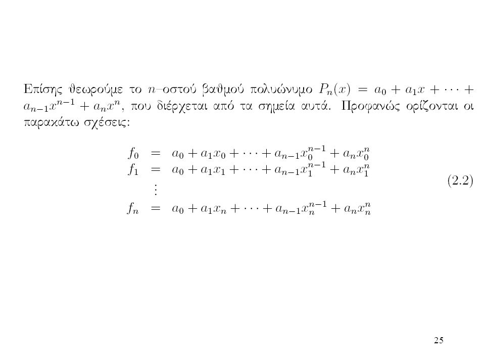
26 Η ορίζουσα αυτή είναι διαφορετική από το μηδέν, επομένως το σύστημα (2
Η ορίζουσα αυτή είναι διαφορετική από το μηδέν, επομένως το σύστημα (2.2) έχει μοναδική λύση και το πολυώνυμο Pn(x) είναι μοναδικό.

27 ΒΙΒΛΙΟΓΡΑΦΙΑ: ΠΑΝΕΠΙΣΤΗΜΙΟ ΙΩΑΝΝΙΝΩΝ, ΕΠΙΣΤΗΜΟΝΙΚΟΙ ΥΠΟΛΟΓΙΣΜΟΙ, Μιχάλης Τζούμας

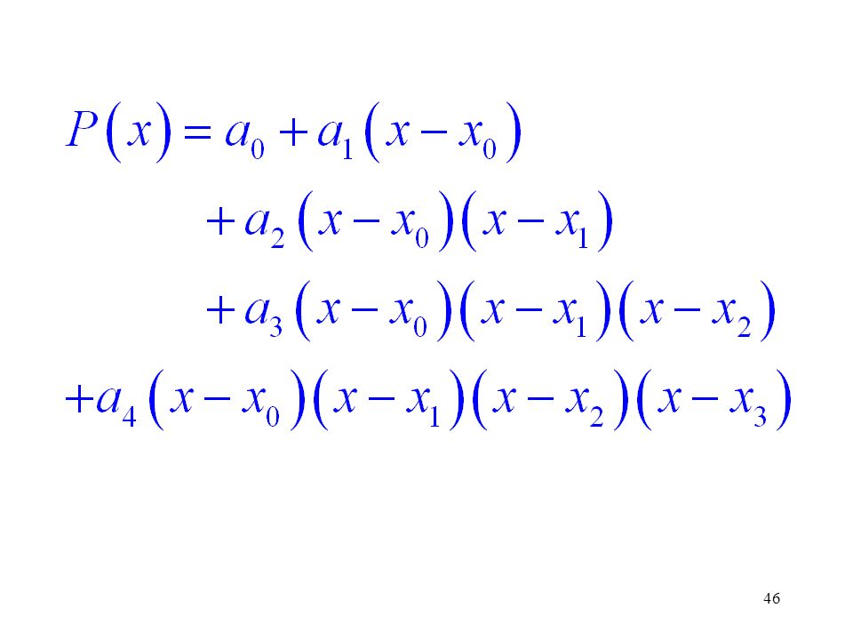
28 Lagrange Polynomials The formula used to interpolate between data pairs (x0,f(x0)), (x1,f(x1)),…, (xn,f(xn)) is given by, Where the polynomial Pj(x) is given by,

29 Lagrange Polynomials In general,

30 Lagrange Polynomials Consider the table of interpolating points we wish to fit. i x f(x) x0 f(x0) 1 x1 f(x1) 2 x2 f(x2) 3 x3 f(x3)

31 Lagrange Polynomials The interpolation polynomial is, i x f(x) x0
x0 f(x0) 1 x1 f(x1) 2 x2 f(x2) 3 x3 f(x3) The interpolation polynomial is,

32 Advantages / Disadvantages
The Lagrange formula is popular because it is well known and is easy to code. Also, the data are not required to be specified with x in ascending or descending order. Although the computation of Pn(x) is simple, the method is still not particularly efficient for large values of n. When n is large and the data for x is ordered, some improvement in efficiency can be obtained by considering only the data pairs in the vicinity of the x value for which Pn(x) is sought. The price of this improved efficiency is the possibility of a poorer approximation to Pn(x).

33 Diagram showing Interpolation (incrementally from one to 5 points)

34 Μέθοδος Διηρημένων Διαφορών Newton
Υπάρχουν περιπτώσεις κατά τις οποίες είναι δυνατόν να προστίθενται νέα σημεία στα ήδη υπάρχοντα που έχουν προσεγγιστεί με κάποια αριθμητική μέθοδο. Στην περίπτωση της παρεμβολής Lagrange (πολυωνυμική παρεμβολή) η συνάρτηση (πολυώνυμο παρεμβολής) που προκύπτει δεν μπορεί να χρησιμοποιηθεί για κάθε νέα τιμή που προστίθεται και πρέπει να υπολογιστεί εκ νέου (επιπτώσεις : δαπάνη υπολογιστικού χρόνου και αύξηση του κόστους υπολογισμών). Η μέθοδος διηρημένων διαφορών Newton επιλύει αυτό το πρόβλημα χρησιμοποιώντας μία ήδη υπολογισμένη συνάρτηση παρεμβολής και διορθώνοντάς την, λαμβάνοντας υπόψη κάθε νέο σημείο που μπορεί να προστεθεί.

35 Στην περίπτωση της μεθόδου Newton το πολυώνυμο παρεμβολής έχει τη μορφή:
Αν λάβουμε τα ai έτσι ώστε Pn(x) = ƒ(x) σε n+1 γνωστά σημεία έτσι ώστε Pn(xi) = ƒ(xi), i=0,1,…,n, τότε το Pn(x) είναι ένα πολυώνυμο παρεμβολής.

36 Newton’s Divided differences
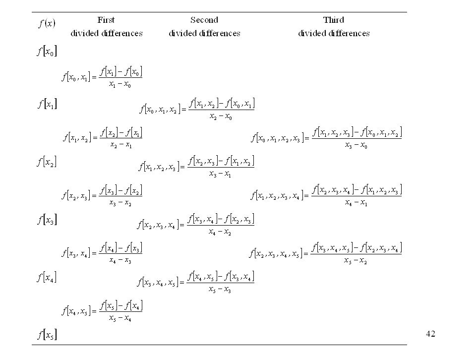
A divided difference is defined as the difference in the function values at two points, divided by the difference in the values of the corresponding independent variable. Thus, the first divided difference at point is defined as The second difference is given as: In general,

37 Divided differences and the coefficients
The divided difference of a function, with respect to is denoted as It is called as zeroth divided difference and is simply the value of the function, at

38 The divided difference of a function,
called as the first divided difference, is denoted with respect to and

39 The divided difference of a function,
called as the second divided difference, is denoted as with respect to and ,

40 The third divided difference with respect to
, and

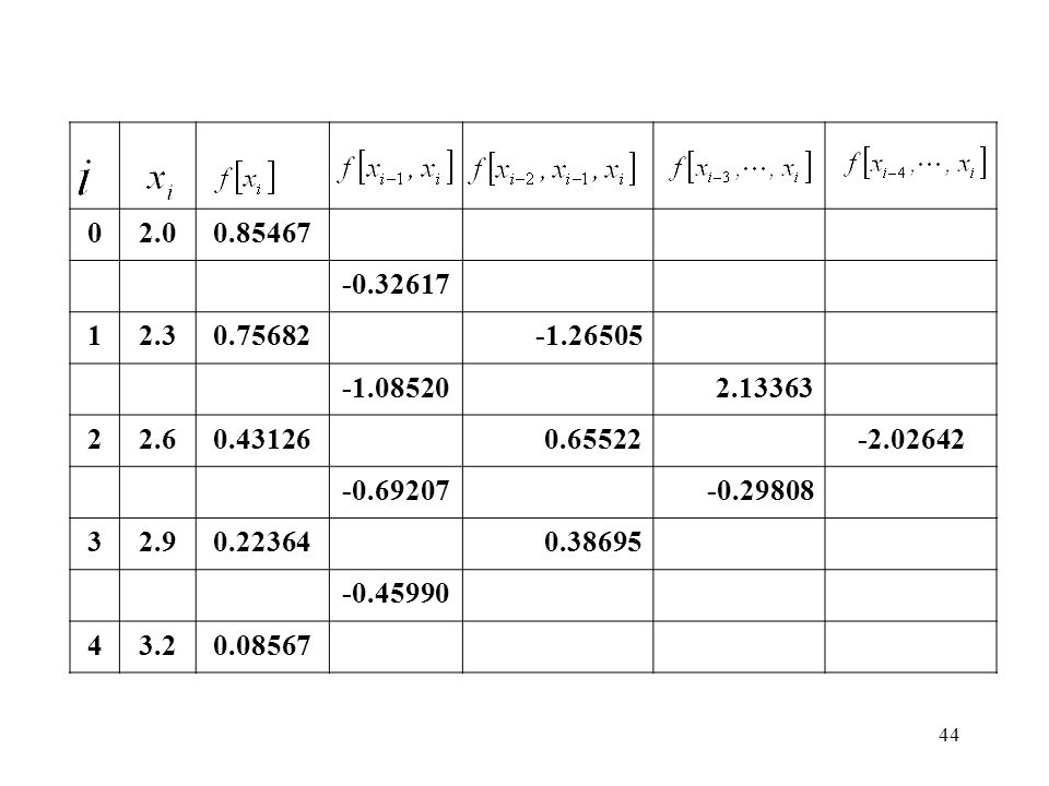
41 The coefficients of Newton’s interpolating polynomial are:
and so on.

42

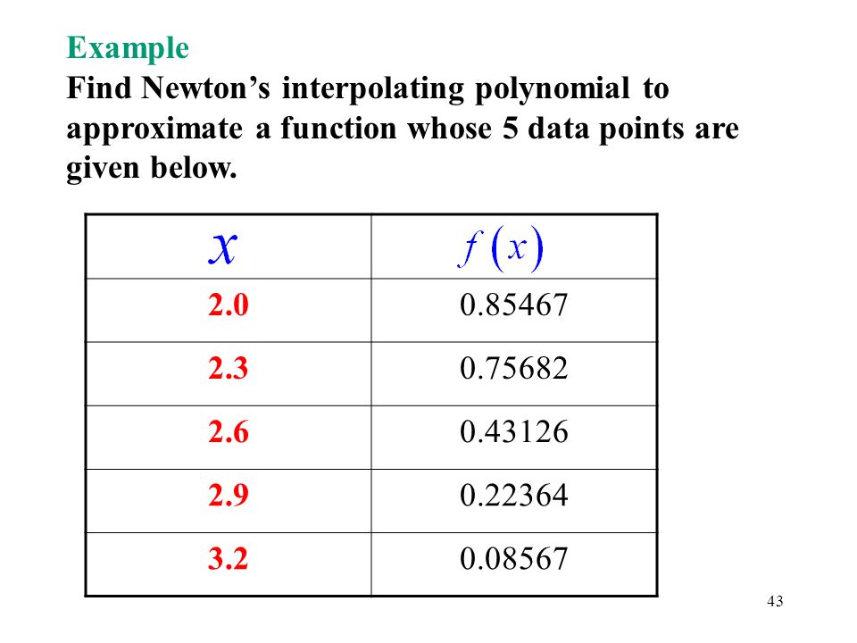
43 Example Find Newton’s interpolating polynomial to approximate a function whose 5 data points are given below. 2.0 2.3 2.6 2.9 3.2

44 2.0 1 2.3 2 2.6 3 2.9 4 3.2

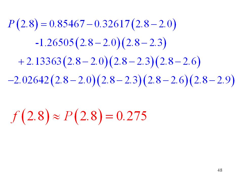
45 The 5 coefficients of the Newton’s interpolating polynomial are:

46

47 P(x) can now be used to estimate the value of the function f(x) say at x = 2.8.

48

49 Παράδειγμα

50 The 3rd degree polynomial fitting all points from x0 = 3. 2 to x3 = 4
The 3rd degree polynomial fitting all points from x0 = 3.2 to x3 = 4.8 is given by P3(x) = (x - 3.2) (x - 3.2)(x - 2.7) – 0.528(x - 3.2)(x - 2.7)(x - 1.0) The 4th degree polynomial fitting all points is given by P4(x) = P3(x) (x - 3.2)(x - 2.7)(x - 1.0)(x - 4.8) The interpolated value at x = 3.0 gives P3(x) =

51 Newton’s Divided-Difference Interpolating Polynomials
Linear Interpolation Connecting two data points with a straight line f1(x) designates a first-order interpolating polynomial. Slope Linear-interpolation formula

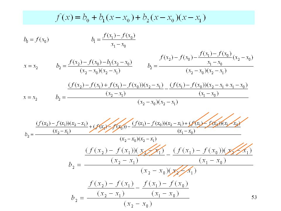
52 Quadratic Interpolation
If three (3) data points are available, the estimate is improved by introducing some curvature into the line connecting the points. A second-order polynomial (parabola) can be used for this purpose A simple procedure can be used to determine the values of the coefficients Represents a second order polynomial Could you figure out how to derive this using the above equation?

53

54 General Form of Newton’s Interpolating Polynomials
Bracketed function evaluations are finite divided differences

55 DIVIDED DIFFERENCE TABLE
EXAMPLE xi f(xi) x0 f(x0) x1 f(x1) x2 f(x2) x3 f(x3) x4 f(x4) f[xi,xj] f[x1,x0] f[x2,x1] f[x3,x2] f[x4,x3] f[xi,xj,xk] f[x2,x1,x0] f[x3,x2,x1] f[x4,x3,x2] f[x,x,x,x] f[x3,x2,x1,x0] f[x4,x3,x2,x1] xi f(xi) x0=0 2 x1=2 14 x2=3 74 x3=4 242 x4=5 602 f[xi,xj] 6 60 168 360 f[xi,xj,xk] 18 54 96 f[x,x,x,x] 9 14 f[x...x] 1 f1(x) = 2 + 6*(x-0) (based on x0 and x1) f2(x) = 2 + 6*(x-0)+18(x-0)(x-2) (based on x0, x1 and x2) f3(x) = 2 + 6*(x-0)+18(x-0)(x-2)+9(x-0)(x-2)(x-3) (based on x0, x1, x2, and x3) f4(x) = 2 + 6x +18x(x-2) +9x(x-2)(x-3) +1x(x-2)(x-3)(x-4) (based on x0, x1, x2, x3, and x4) = x4 – x2 + 2

56 f(x) = 0.58(x-1) -0.057(x-1)(x-2.72) x0=1 f(x0)=ln(1) = 0
Given: x0=1 f(x0)=ln(1) = 0 x1=e f(x1)=ln(2.72) = 1 x2=e2 f(x2)=ln(7.39) = 2 Estimate ln(2) = ? using interpolation Find f(x) first xi f(xi) x0=1 x1=2.72 1 x2=7.39 2 f[xi,xj] .58 .214 f[xi,xj xk] -.057 f(x) = 0.58(x-1) -0.057(x-1)(x-2.72) Then calculate f(2)=0.58(2-1)-0.057(2-1)(2-2.72) = 0.621 [ TRUE ln(2) = ]

57 Yet Another Example: f(x) = 0.462(x-1) -0.052(x-1)(x-4)
Given: x0=1 f(x0)=ln(1)=0 x1=4 f(x1)=ln(4)=1.386 x2=6 f(x2)=ln(6)=1.791 Estimate ln(2) = ? using interpolation Find f(x) first xi f(xi) x0=1 x1=4 1.386 x2=6 1.79 f[xi,xj] .462 .2025 f[xi,xj xk] -.052 f(x) = 0.462(x-1) -0.052(x-1)(x-4) Then calculate f(2)=0.462*(2-1) *(2-1)(2-4) = 0.566 [ TRUE ln(2) = ]

58 Error Estimation in Newton’s Interpolating Polynomials
Structure of interpolating polynomials is similar to the Taylor series expansion, i.e. finite divided differences are added sequentially to capture the higher order derivatives. For an nth-order interpolating polynomial, an analogous relationship for the error is: If an additional point (xn+1 , f(xn+1)) is available, then This result is based on the assumption that the series is strongly convergent. i.e. (n+1)th-order prediction is closer to the true value than the nth-order prediction.

59 which is half of the true error (same order of magnitude).
Previous Example: x0=1 f(x0)=ln(1) = 0 x1=e f(x1)=ln(2.72) = 1 x2=e2 f(x2)=ln(7.39) = 2 f(x) = 0.58(x-1) -0.057(x-1)(x-2.72) f(2) = 0.621 Example (for computing error): In the previous Example, add a fourth point x3=4 f(x3) = 1.386 And estimate the approximate error in computing ln(2) 2nd order polynomial estimation: f(2) = 0.621 True error = ln(2) – f(2) = = 0.072 R2 = f3(x) - f2(x) = f[ x3, x2, x1, x0] (x- x0)(x- x1)(x- x2) or R2= 0.011*(x-1)(x-2.72)(x-7.39) If we plug-in x=2 in the above expression, we get: R2= 0.011*(2-1)(2-2.72)(2-7.39)= 0.042 which is half of the true error (same order of magnitude).

60 which is half of the true error (same order of magnitude).
Previous Example: x0= f(x0)=0 x1= f(x1)=1.386 x2= f(x2)=1.791 f(x) = 0.462(x-1) -0.052(x-1)(x-4) f(2) = 0.566 Example (for computing error): In the previous Example, add a fourth point x3= f(x3) = 1.609 And estimate the error in computing ln(2)= f(2) 2nd order polynomial estimation: f(2) = 0.566 True error = ln(2) – f(2) = = 0.127 R2= f3(x)-f2(x) = f[ x3, x2, x1, x0] (x- x0)(x- x1)(x- x2) or R2= 0.008*(x- 1)(x- 4)(x- 6) If we plug-in x=2 in the above expression, we get: R2= 0.008*(2- 1)(2- 4)(2- 6) = 0.064 which is half of the true error (same order of magnitude).

61 Newton Interpolation Pseudo Code

62 Features of Newton Divided-Differences to get Interpolating Polynomial
Data need not be equally spaced Arrangement of data does not have to be ascending or descending, but it does influence error of interpolation Best case is when the base points are close to the unknown value Estimate of relative error: Error estimate for nth-order polynomial is the difference between the (n+1)th and nth-order prediction.

63 Άσκηση Determine ln(2) using the following table

64 Lagrange Interpolating Polynomials
The Lagrange interpolating polynomial is simply a reformulation of the Newton’s polynomial that avoids the computation of divided differences: Above formula can be easily verified by plugging in x0, x1…in the equation one at a time and checking if the equality is satisfied.

65 A visual depiction of the rationale behind the Lagrange polynomial
A visual depiction of the rationale behind the Lagrange polynomial . The figure shows a second order case: Each of the three terms passes through one of the data points and zero at the other two. The summation of the three terms must, therefore, be unique second order polynomial f2(x) that passes exactly through three points.

66 Coefficients of an Interpolating Polynomial
Although both the Newton and Lagrange polynomials are well suited for determining intermediate values between points, they do not provide a polynomial in conventional form: Since n+1 data points are required to determine n+1 coefficients, simultaneous linear systems of equations can be used to calculate “a”s. Where “x”s are the knowns and “a”s are the unknowns. Time complexity for Newton’s: O(n2) vs. Gaussian Elim. O(n3)

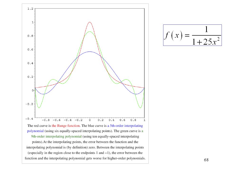
67 Οι κίνδυνοι της πολυωνυμικής παρεμβολής
Έχει παρατηρηθεί ότι όσο μεγαλώνει ο βαθμός του πολυωνύμου παρεμβολής τότε η παρεμβολή δεν είναι επιτυχής, δηλ. οι εκτιμήσεις για την τιμή της συνάρτησης είναι ιδιαίτερα μη ακριβείς (συνήθως παρατηρούνται γρήγορες ταλαντώσεις στις τιμές του πολυωνύμου). In the mathematical field of numerical analysis, Runge's phenomenon is a problem of oscillation at the edges of an interval that occurs when using polynomial interpolation with polynomials of high degree over a set of equispaced interpolation points. It was discovered by Carl David Tolmι Runge when exploring the behavior of errors when using polynomial interpolation to approximate certain functions. The discovery was important because it shows that going to higher degrees does not always improve accuracy.

68

69 Προσέγγιση κατά τμήματα με πολυώνυμα ελάχιστου βαθμού

70 Προσέγγιση με spline Η καμπύλη spline στα μαθηματικά είναι ένα πολυώνυμο που ορίζεται τμηματικά από πολυώνυμα χαμηλού βαθμού, αλλά όχι του ελάχιστου δυνατού, με συνεχείς παραγώγους στα σημεία (κόμβοι) που αυτά ενώνονται. Η συγκεκριμένη καμπύλη αποφεύγει να χρησιμοποιήσει πολυώνυμα μεγάλου βαθμού (άρα δεν εμφανίζονται αφύσικες ταλαντώσεις στα διαστήματα μεταξύ των σημείων). Επιπλέον η προσέγγιση δεν γίνεται με τα πολυώνυμα ελάχιστου βαθμού και έτσι αποφεύγονται οι ασυνέχειες στις παραγώγους στους κόμβους. Η φυσική («κυβική») spline είναι η συχνότερα χρησιμοποιούμενη καμπύλη.

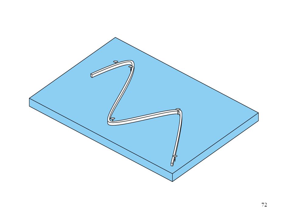
71 Spline Interpolation linear spline  
There are cases where polynomials can lead to erroneous results because of round off error and overshoot. Alternative approach is to apply lower-order polynomials to subsets of data points. Such connecting polynomials are called spline functions. EXAMPLE: spline fits for a set of 4 points: (a) linear (b) quadratic (c) cubic splines linear spline   is superior to higher-order interpolating polynomials (parts a, b, and c)

72

73 Quadratic Spline example

74 Quadratic Splines - Equations
Given (n+1) points, there are 3(n) coefficients to find and hence, need to determine 3n equations to solve: Each polynomial must pass through the endpoints of the interval that they are associated with. And these conditions result in 2n equations: The first derivatives at the interior knots must be equal ((n-1) equations): So far, we are one equation short. Since the last equation will be derived using only 2 points, it must be a line equation with only bn and cn to be determined (an = 0)