ΠΑΝΕΠΙΣΤΗΜΙΟ ΙΩΑΝΝΙΝΩΝ ΑΝΟΙΚΤΑ ΑΚΑΔΗΜΑΪΚΑ ΜΑΘΗΜΑΤΑ Εξόρυξη Δεδομένων Απορροφητικοί τυχαίοι περίπατοι. Προβλήματα κάλυψης Διδάσκων: Επίκ. Καθ. Παναγιώτης.

Παρουσίαση με θέμα: "ΠΑΝΕΠΙΣΤΗΜΙΟ ΙΩΑΝΝΙΝΩΝ ΑΝΟΙΚΤΑ ΑΚΑΔΗΜΑΪΚΑ ΜΑΘΗΜΑΤΑ Εξόρυξη Δεδομένων Απορροφητικοί τυχαίοι περίπατοι. Προβλήματα κάλυψης Διδάσκων: Επίκ. Καθ. Παναγιώτης."— Μεταγράφημα παρουσίασης:

1 ΠΑΝΕΠΙΣΤΗΜΙΟ ΙΩΑΝΝΙΝΩΝ ΑΝΟΙΚΤΑ ΑΚΑΔΗΜΑΪΚΑ ΜΑΘΗΜΑΤΑ Εξόρυξη Δεδομένων Απορροφητικοί τυχαίοι περίπατοι. Προβλήματα κάλυψης Διδάσκων: Επίκ. Καθ. Παναγιώτης Τσαπάρας

2 Άδειες Χρήσης Το παρόν εκπαιδευτικό υλικό υπόκειται σε άδειες χρήσης Creative Commons. Για εκπαιδευτικό υλικό, όπως εικόνες, που υπόκειται σε άλλου τύπου άδειας χρήσης, η άδεια χρήσης αναφέρεται ρητώς.

3 DATA MINING LECTURE 14 Absorbing Random walks Coverage

4 Random Walks on Graphs

5 Random walk

6 Stationary distribution

7 Random walk with Restarts This is the random walk used by the PageRank algorithm At every step with probability 1-α do a step of the random walk (follow a random link). With probability α restart the random walk from a randomly selected node. The effect of the restart is that paths followed are never too long. In expectation paths have length 1/α. Restarts can also be from a specific node in the graph (always start the random walk from there). What is the effect of that? The nodes that are close to the starting node have higher probability to be visited. The probability defines a notion of proximity between the starting node and all the other nodes in the graph.

8 ABSORBING RANDOM WALKS

9 Random walk with absorbing nodes What happens if we do a random walk on this graph? What is the stationary distribution? All the probability mass on the red sink node: The red node is an absorbing node.

10 Random walk with absorbing nodes What happens if we do a random walk on this graph? What is the stationary distribution? There are two absorbing nodes: the red and the blue. The probability mass will be divided between the two.

11 Absorption probability If there are more than one absorbing nodes in the graph a random walk that starts from a non- absorbing node will be absorbed in one of them with some probability. The probability of absorption gives an estimate of how close the node is to red or blue.

12 Absorption probability Computing the probability of being absorbed: The absorbing nodes have probability 1 of being absorbed in themselves and zero of being absorbed in another node. For the non-absorbing nodes, take the (weighted) average of the absorption probabilities of your neighbors if one of the neighbors is the absorbing node, it has probability 1. Repeat until convergence (= very small change in probs). 2 2 1 1 1 2 1

13 Absorption probability Computing the probability of being absorbed: The absorbing nodes have probability 1 of being absorbed in themselves and zero of being absorbed in another node. For the non-absorbing nodes, take the (weighted) average of the absorption probabilities of your neighbors if one of the neighbors is the absorbing node, it has probability 1. Repeat until convergence (= very small change in probs). 2 2 1 1 1 2 1

14 Why do we care? Why do we care to compute the absorption probability to sink nodes? Given a graph (directed or undirected) we can choose to make some nodes absorbing. Simply direct all edges incident on the chosen nodes towards them and remove outgoing edges. The absorbing random walk provides a measure of proximity of non-absorbing nodes to the chosen nodes. Useful for understanding proximity in graphs. Useful for propagation in the graph. E.g, some nodes have positive opinions for an issue, some have negative, to which opinion is a non-absorbing node closer?

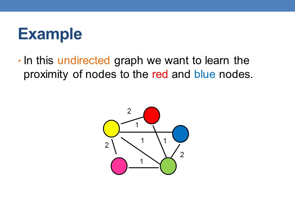
15 Example In this undirected graph we want to learn the proximity of nodes to the red and blue nodes. 2 2 1 1 1 2 1

16 Example Make the nodes absorbing. 2 2 1 1 1 2 1

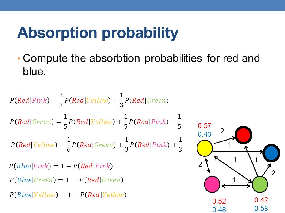
17 Absorption probability Compute the absorbtion probabilities for red and blue. 0.52 0.48 0.42 0.58 0.57 0.43 2 2 1 1 1 2 1

18 Penalizing long paths The orange node has the same probability of reaching red and blue as the yellow one. Intuitively though it is further away. 0.52 0.48 0.42 0.58 0.57 0.43 2 2 1 1 1 2 1 1 0.57 0.43

19 Penalizing long paths Add an universal absorbing node to which each node gets absorbed with probability α. 1-α α α α α With probability α the random walk dies With probability (1-α) the random walk continues as before. The longer the path from a node to an absorbing node the more likely the random walk dies along the way, the lower the absorbtion probability. e.g.

20 Random walk with restarts Adding a jump with probability α to a universal absorbing node seems similar to Pagerank. Random walk with restart: Start a random walk from node u. At every step with probability α, jump back to u. The probability of being at node v after large number of steps defines again a similarity between nodes u,v. The Random Walk With Restarts (RWS) and Absorbing Random Walk (ARW) are similar but not the same RWS computes the probability of paths from the starting node u to a node v, while AWR the probability of paths from a node v, to the absorbing node u. RWS defines a distribution over all nodes, while AWR defines a probability for each node. An absorbing node blocks the random walk, while restarts simply bias towards starting nodes Makes a difference when having multiple (and possibly competing) absorbing nodes.

21 Propagating values Assume that Red has a positive value and Blue a negative value Positive/Negative class, Positive/Negative opinion. We can compute a value for all the other nodes by repeatedly averaging the values of the neighbors The value of node u is the expected value at the point of absorption for a random walk that starts from u. +1 0.05 -0.16 0.16 2 2 1 1 1 2 1

22 Electrical networks and random walks Our graph corresponds to an electrical network. There is a positive voltage of +1 at the Red node, and a negative voltage -1 at the Blue node. There are resistances on the edges inversely proportional to the weights (or conductance proportional to the weights). The computed values are the voltages at the nodes. +1 2 2 1 1 1 2 1 0.05 -0.16 0.16

23 Opinion formation

24 Example Social network with internal opinions. 2 2 1 1 1 2 1 s = +0.5 s = -0.3 s = -0.1s = +0.2 s = +0.8

25 Example 2 2 1 1 1 2 1 1 1 1 1 1 s = +0.5 s = -0.3 s = -0.1 s = -0.5 s = +0.8 The external opinion for each node is computed using the value propagation we described before Repeated averaging. Intuitive model: my opinion is a combination of what I believe and what my social network believes. One absorbing node per user with value the internal opinion of the user. One non-absorbing node per user that links to the corresponding absorbing node. z = +0.22 z = +0.17 z = -0.03 z = 0.04 z = -0.01

26 Hitting time A related quantity: Hitting time H(u,v) The expected number of steps for a random walk starting from node u to end up in v for the first time Make node v absorbing and compute the expected number of steps to reach v. Assumes that the graph is strongly connected, and there are no other absorbing nodes. Commute time H(u,v) + H(v,u): often used as a distance metric Proportional to the total resistance between nodes u, and v.

27 Transductive learning If we have a graph of relationships and some labels on some nodes we can propagate them to the remaining nodes Make the labeled nodes to be absorbing and compute the probability for the rest of the graph. E.g., a social network where some people are tagged as spammers. E.g., the movie-actor graph where some movies are tagged as action or comedy. This is a form of semi-supervised learning We make use of the unlabeled data, and the relationships. It is also called transductive learning because it does not produce a model, but just labels the unlabeled data that is at hand. Contrast to inductive learning that learns a model and can label any new example.

28 Implementation details

29 COVERAGE

30 Example Promotion campaign on a social network We have a social network as a graph. People are more likely to buy a product if they have a friend who has the product. We want to offer the product for free to some people such that every person in the graph is covered: they have a friend who has the product. We want the number of free products to be as small as possible.

31 Example One possible selection Promotion campaign on a social network We have a social network as a graph. People are more likely to buy a product if they have a friend who has the product. We want to offer the product for free to some people such that every person in the graph is covered: they have a friend who has the product. We want the number of free products to be as small as possible

32 Example A better selection Promotion campaign on a social network We have a social network as a graph. People are more likely to buy a product if they have a friend who has the product. We want to offer the product for free to some people such that every person in the graph is covered: they have a friend who has the product. We want the number of free products to be as small as possible

33 Dominating set

34 Set Cover

35 Applications Suppose that we want to create a catalog (with coupons) to give to customers of a store: We want for every customer, the catalog to contain a product bought by the customer (this is a small store). How can we model this as a set cover problem?

36 Applications coke beer milk coffee tea

37 Applications coke beer milk coffee tea

38 Applications coke beer milk coffee tea

39 Applications

40 Best selection variant

41 Complexity Both the Set Cover and the Maximum Coverage problems are NP-complete What does this mean? Why do we care? There is no algorithm that can guarantee to find the best solution in polynomial time Can we find an algorithm that can guarantee to find a solution that is close to the optimal? Approximation Algorithms.

42 Approximation Algorithms For an (combinatorial) optimization problem, where: X is an instance of the problem, OPT(X) is the value of the optimal solution for X, ALG(X) is the value of the solution of an algorithm ALG for X. ALG is a good approximation algorithm if the ratio of OPT(X) and ALG(X) is bounded for all input instances X. Minimum set cover: X = G is the input graph, OPT(G) is the size of minimum set cover, ALG(G) is the size of the set cover found by an algorithm ALG. Maximum coverage: X = (G,k) is the input instance, OPT(G,k) is the coverage of the optimal algorithm, ALG(G,k) is the coverage of the set found by an algorithm ALG.

43 Approximation Algorithms

44

45 A simple approximation ratio for set cover Any algorithm for set cover has approximation ratio  = |S max |, where S max is the set in S with the largest cardinality Proof: OPT(X)≥N/|S max |  N ≤ |S max |OPT(X) ALG(X) ≤ N ≤ |S max |OPT(X) This is true for any algorithm. Not a good bound since it can be that |S max |=O(N).

46 An algorithm for Set Cover What is the most natural algorithm for Set Cover? Greedy: each time add to the collection C the set S i from S that covers the most of the remaining elements.

47 The GREEDY algorithm

48 Greedy is not always optimal coke beer milk coffee tea coke beer milk coffee tea OptimalGreedy

49 Greedy is not always optimal coke beer milk coffee tea coke beer milk coffee tea OptimalGreedy

50 Greedy is not always optimal coke beer milk coffee tea coke beer milk coffee tea OptimalGreedy

51 Greedy is not always optimal coke beer milk coffee tea coke beer milk coffee tea OptimalGreedy

52 Greedy is not always optimal coke beer milk coffee tea coke beer milk coffee tea OptimalGreedy

53 Greedy is not always optimal Selecting Coke first forces us to pick coffee as well. Milk and Beer cover more customers together. coke beer milk coffee tea coke beer milk coffee tea

54 Approximation ratio of GREEDY OPT(X) = 2 GREEDY(X) = logN  =½logN

55 Maximum Coverage What is a reasonable algorithm?

56 Approximation Ratio for Max-K Coverage

57 Proof of approximation ratio

58 Optimizing submodular functions True for any monotone and submodular set function!

59 Other variants of Set Cover Hitting Set: select a set of elements so that you hit all the sets (the same as the set cover, reversing the roles). Vertex Cover: Select a subset of vertices such that you cover all edges (an endpoint of each edge is in the set) There is a 2-approximation algorithm. Edge Cover: Select a set of edges that cover all vertices (there is one edge that has endpoint the vertex) There is a polynomial algorithm.

60 OVERVIEW

61 Class Overview In this class you saw a set of tools for analyzing data Frequent Itemsets, Association Rules. Sketching. Recommendation Systems. Clustering. Minimum Description Length. Singular Value Decomposition. Classification. Link Analysis Ranking. Random Walks. Coverage. All these are useful when trying to make sense of the data. A lot more tools exist. I hope that you found this interesting, useful and fun.

62 Τέλος Ενότητας

63 Χρηματοδότηση Το παρόν εκπαιδευτικό υλικό έχει αναπτυχθεί στα πλαίσια του εκπαιδευτικού έργου του διδάσκοντα. Το έργο «Ανοικτά Ακαδημαϊκά Μαθήματα στο Πανεπιστήμιο Ιωαννίνων» έχει χρηματοδοτήσει μόνο τη αναδιαμόρφωση του εκπαιδευτικού υλικού. Το έργο υλοποιείται στο πλαίσιο του Επιχειρησιακού Προγράμματος «Εκπαίδευση και Δια Βίου Μάθηση» και συγχρηματοδοτείται από την Ευρωπαϊκή Ένωση (Ευρωπαϊκό Κοινωνικό Ταμείο) και από εθνικούς πόρους.

64 Σημειώματα

65 Σημείωμα Ιστορικού Εκδόσεων Έργου Το παρόν έργο αποτελεί την έκδοση 1.0. Έχουν προηγηθεί οι κάτωθι εκδόσεις: Έκδοση 1.0 διαθέσιμη εδώ. http://ecourse.uoi.gr/course/view.php?id=1051. http://ecourse.uoi.gr/course/view.php?id=1051

66 Σημείωμα Αναφοράς Copyright Πανεπιστήμιο Ιωαννίνων, Διδάσκων: Επίκ. Καθ. Παναγιώτης Τσαπάρας. «Εξόρυξη Δεδομένων. Απορροφητικοί τυχαίοι περίπατοι. Προβλήματα κάλυψης». Έκδοση: 1.0. Ιωάννινα 2014. Διαθέσιμο από τη δικτυακή διεύθυνση: http://ecourse.uoi.gr/course/view.php?id=1051. http://ecourse.uoi.gr/course/view.php?id=1051

67 Σημείωμα Αδειοδότησης Το παρόν υλικό διατίθεται με τους όρους της άδειας χρήσης Creative Commons Αναφορά Δημιουργού - Παρόμοια Διανομή, Διεθνής Έκδοση 4.0 [1] ή μεταγενέστερη. [1] https://creativecommons.org/licenses/by-sa/4.0/https://creativecommons.org/licenses/by-sa/4.0/