Κατέβασμα παρουσίασης
Η παρουσίαση φορτώνεται. Παρακαλείστε να περιμένετε

1
DATA MINING LECTURE 6 Mixture of Gaussians and the EM algorithm
DBSCAN: A Density-Based Clustering Algorithm Clustering Validation

2
Ανακοινώσεις Η προθεσμία για τη παράδοση των θεωρητικών ασκήσεων είναι Τετάρτη 4/4 Καθυστερημένες ασκήσεις σε μετέπειτα ημέρες θα πρέπει να παραδοθούν στην κα. Σουλίου, η οποία θα σημειώνει την ημέρα παράδοσης (Πέμπτη-Παρασκευή μέχρι τις 2:30, ή κάτω από την πόρτα μετά). Μπορείτε να τις παραδώσετε και ηλεκτρονικά αν θέλετε. WEKA: Αν σας βγάλει out-of-memory error, ακολουθείστε τις οδηγίες και αλλάξτε το .ini αρχείο. Θα σας πει ότι δεν επιτρέπεται, οπότε πρέπει να το αντιγράψετε αλλού να το αλλάξετε και μετά να το αντιγράψετε ξανά. LSH Implementation: Για την υλοποίηση θα χρειαστείτε μια υλοποίηση ενός Dictionary και List. Η C++ έχει μια βιβλιοθήκη (STL), και η Java τα έχει ως built-in data types.
. Μπορείτε να τις παραδώσετε και ηλεκτρονικά αν θέλετε. WEKA: Αν σας βγάλει out-of-memory error, ακολουθείστε τις οδηγίες και αλλάξτε το .ini αρχείο. Θα σας πει ότι δεν επιτρέπεται, οπότε πρέπει να το αντιγράψετε αλλού να το αλλάξετε και μετά να το αντιγράψετε ξανά. LSH Implementation: Για την υλοποίηση θα χρειαστείτε μια υλοποίηση ενός Dictionary και List. Η C++ έχει μια βιβλιοθήκη (STL), και η Java τα έχει ως built-in data types.")
3
Συντομο Μαθημα για HASH TABLE IMPLEMENTATIONS

4
Vector, map Container Χαρακτηριστικά vector Δυναμικός πίνακας map
Κρατάει ζεύγη κλειδιών και τιμών (key-value pairs). Συσχετίζει αντικείμενα-κλειδιά με αντικείμενα-τιμές. Το κάθε κλειδί μπορεί να συσχετίζεται με μόνο μία τιμή
. Συσχετίζει αντικείμενα-κλειδιά με αντικείμενα-τιμές. Το κάθε κλειδί μπορεί να συσχετίζεται με μόνο μία τιμή.")
5
vector Μέθοδος Λειτουργία size()
επιστρέφει τον αριθμό των στοιχείων μέσα στον πίνακα push_back() προσθέτει ένα στοιχείο στο τέλος του πίνακα pop_back() αφαιρεί το τελευταίο στοιχείο του πίνακα back() επιστρέφει το τελευταίο στοιχείο του πίνακα operator [] τυχαία πρόσβαση στα στοιχεία του πίνακα empty() επιστρέφει true αν το vector είναι άδειο insert() προσθέτει ένα στοιχείο σε ενδιάμεση θέση (χρησιμοποιώντας iterator) erase() αφαιρεί ένα στοιχείο από ενδιάμεση θέση (χρησιμοποιώντας iterator)
 προσθέτει ένα στοιχείο στο τέλος του πίνακα. pop_back() αφαιρεί το τελευταίο στοιχείο του πίνακα. back() επιστρέφει το τελευταίο στοιχείο του πίνακα. operator [] τυχαία πρόσβαση στα στοιχεία του πίνακα. empty() επιστρέφει true αν το vector είναι άδειο. insert() προσθέτει ένα στοιχείο σε ενδιάμεση θέση (χρησιμοποιώντας iterator) erase() αφαιρεί ένα στοιχείο από ενδιάμεση θέση (χρησιμοποιώντας iterator)")
6
Παράδειγμα #include <iostream> #include <vector>
using namespace std; int main(){ vector<int> v; int x; do{ cin >> x; v.push_back(x); }while (x != -1); v[v.size() - 1] = 0; cout << "vector elements: "; for (int i = 0; i < v.size(); i ++){ cout << v[i] << " "; } cout << endl;
{ vector<int> v; int x; do{ cin >> x; v.push_back(x); }while (x != -1); v[v.size() - 1] = 0; cout << vector elements: ; for (int i = 0; i < v.size(); i ++){ cout << v[i] << ; } cout << endl;")
7
Παραδειγμα map #include <iostream> #include <map>
using namespace std; int main(){ map<string,Person*> M; string fname,lname; while (!cin.eof()){ cin >> fname >> lname; Person *p =new Person(fname,lname); M[lname] = p; } map<string,Person*>::iterator iter = M.find(“marley"); if (iter == M.end()){ cout << “marley is not in\n"; }else{ M[“marley"]->PrintPersonalDetails();
{ map<string,Person*> M; string fname,lname; while (!cin.eof()){ cin >> fname >> lname; Person *p =new Person(fname,lname); M[lname] = p; } map<string,Person*>::iterator iter = M.find( marley ); if (iter == M.end()){ cout << marley is not in\n ; }else{ M[ marley ]->PrintPersonalDetails();")
8
Iterators map #include <iostream> #include <map> using namespace std; int main(){ map<string,Person*> M; string fname,lname; while (!cin.eof()){ cin >> fname >> lname; Person *p =new Person(fname,lname); M[lname] = p; } map<string,Person*>::iterator iter; for (iter = M.begin(); iter != M.end(); i++){ cout << (*iter).first << “:”; (*iter).second->PrintPersonalDetails(); (*iter).first: Το κλειδί του map στη θέση στην οποία δείχνει ο iterator (*iter).second: Η τιμή του map στη θέση στην οποία δείχνει ο iterator
){ cin >> fname >> lname; Person *p =new Person(fname,lname); M[lname] = p; } map<string,Person*>::iterator iter; for (iter = M.begin(); iter != M.end(); i++){ cout << (*iter).first << : ; (*iter).second->PrintPersonalDetails(); (*iter).first: Το κλειδί του map στη θέση στην οποία δείχνει ο iterator. (*iter).second: Η τιμή του map στη θέση στην οποία δείχνει ο iterator.")
9
ArrayList O Container ArrayList κληρονομει από το List και αυτό από το Collection. Προσφέρει σειριακή αποθήκευση δεδομένων και έχει όλα τα πλεονεκτήματα και μειονεκτήματα του vector στην C++. Στην Java δεν επιτρέπεται υπερφόρτωση τελεστών οπότε χρησιμοποιούμε την μέθοδο get(index) για να διαβάσουμε ένα στοιχείο. Διάσχιση του ArrayList με την foreach εντολή είναι πιο απλή απ ότι με τον iterator.
 για να διαβάσουμε ένα στοιχείο. Διάσχιση του ArrayList με την foreach εντολή είναι πιο απλή απ ότι με τον iterator.")
10
import java.io.*; import java.util.*; public class arraylist { public static void main(String[] args) { ArrayList<Integer> A = new ArrayList<Integer>(); for (int i = 0; i < 10; i ++){ Random r = new Random(); A.add(r.nextInt(100)); System.out.println(A.get(i)); } Collections.sort(A); System.out.println(""); for (int x: A){ System.out.println(x); System.out.println(A.toString());
![import java.io.*; import java.util.*; public class arraylist { public static void main(String[] args) {](http://slideplayer.gr/slide/2296808/8/images/10/import+java.io.%2A%3B+import+java.util.%2A%3B+public+class+arraylist+%7B+public+static+void+main%28String%5B%5D+args%29+%7B.jpg "ArrayList<Integer> A = new ArrayList<Integer>(); for (int i = 0; i < 10; i ++){ Random r = new Random(); A.add(r.nextInt(100)); System.out.println(A.get(i)); } Collections.sort(A); System.out.println( ); for (int x: A){ System.out.println(x); System.out.println(A.toString());")
11
HashMap To HashMap ορίζει ένα συνειρμικό αποθηκευτή (associative container) ο οποίος συσχετίζει κλειδιά με τιμές, κληρονομεί από την πιο γενική κλάση Map. Π.χ., ο βαθμός ενός φοιτητή, η συχνότητα με την οποία εμφανίζεται μια λέξη σε ένα κείμενο. H βιβλιοθήκη της Java μας δίνει πιο εύκολη πρόσβαση στα κλειδιά και τις τιμές του map. Χρήσιμες μέθοδοι: put(key,value): προσθέτει ένα νέο key-value ζεύγος containsKey(key): επιστρέφει αληθές αν υπάρχει το κλειδί containsValue(value): επιστρέφει αληθές αν υπάρχει η τιμή values(): επιστρέφει ένα Collection με τις τιμές keySet(): επιστρέφει ένα Set με τις τιμές.
 ο οποίος συσχετίζει κλειδιά με τιμές, κληρονομεί από την πιο γενική κλάση Map. Π.χ., ο βαθμός ενός φοιτητή, η συχνότητα με την οποία εμφανίζεται μια λέξη σε ένα κείμενο. H βιβλιοθήκη της Java μας δίνει πιο εύκολη πρόσβαση στα κλειδιά και τις τιμές του map. Χρήσιμες μέθοδοι: put(key,value): προσθέτει ένα νέο key-value ζεύγος. containsKey(key): επιστρέφει αληθές αν υπάρχει το κλειδί. containsValue(value): επιστρέφει αληθές αν υπάρχει η τιμή. values(): επιστρέφει ένα Collection με τις τιμές. keySet(): επιστρέφει ένα Set με τις τιμές.")
12
import java.io.*; import java.util.*; public class mapexample { public static void main(String[] args) { String line; Map<String,Integer> namesGrades = new HashMap<String,Integer>(); try{ FileReader fr = new FileReader("Files/in.txt"); BufferedReader inReader = new BufferedReader(fr); while((line = inReader.readLine())!=null){ System.out.println(line); String [] words = line.split("\t"); Integer grade = Integer.parseInt(words[1]); namesGrades.put(words[0],grade); } } catch(IOException ex){ System.out.println("IO Error" + ex); for(String x: namesGrades.keySet()){ System.out.println(x + " -- " + namesGrades.get(x));
![import java.io.*; import java.util.*; public class mapexample { public static void main(String[] args) {](http://slideplayer.gr/slide/2296808/8/images/12/import+java.io.%2A%3B+import+java.util.%2A%3B+public+class+mapexample+%7B+public+static+void+main%28String%5B%5D+args%29+%7B.jpg "String line; Map<String,Integer> namesGrades = new HashMap<String,Integer>(); try{ FileReader fr = new FileReader( Files/in.txt ); BufferedReader inReader = new BufferedReader(fr); while((line = inReader.readLine())!=null){ System.out.println(line); String [] words = line.split( \t ); Integer grade = Integer.parseInt(words[1]); namesGrades.put(words[0],grade); } } catch(IOException ex){ System.out.println( IO Error + ex); for(String x: namesGrades.keySet()){ System.out.println(x namesGrades.get(x));")
13
Mixture Models and the EM Algorithm

14
Model-based clustering
In order to understand our data, we will assume that there is a generative process (a model) that creates/describes the data, and we will try to find the model that best fits the data. Models of different complexity can be defined, but we will assume that our model is a distribution from which data points are sampled Example: the data is the height of all people in Greece In most cases, a single distribution is not good enough to describe all data points: different parts of the data follow a different distribution Example: the data is the height of all people in Greece and China We need a mixture model Different distributions correspond to different clusters in the data.
 that creates/describes the data, and we will try to find the model that best fits the data. Models of different complexity can be defined, but we will assume that our model is a distribution from which data points are sampled. Example: the data is the height of all people in Greece. In most cases, a single distribution is not good enough to describe all data points: different parts of the data follow a different distribution. Example: the data is the height of all people in Greece and China. We need a mixture model. Different distributions correspond to different clusters in the data.")
15
Gaussian Distribution
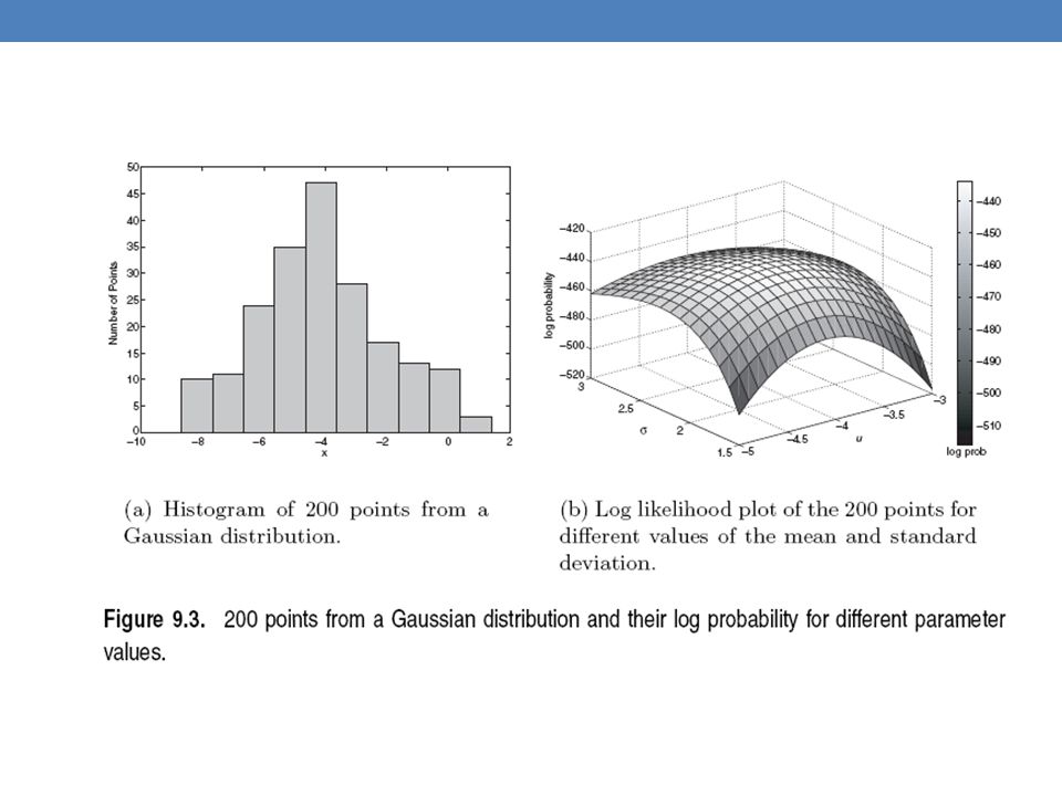
Example: the data is the height of all people in Greece Experience has shown that this data follows a Gaussian (Normal) distribution Reminder: Normal distribution: 𝜇 = mean, 𝜎 = standard deviation 𝑃 𝑥 = 𝜋 𝜎 𝑒 − 𝑥−𝜇 𝜎 2
 distribution. Reminder: Normal distribution: 𝜇 = mean, 𝜎 = standard deviation. 𝑃 𝑥 = 1 2𝜋 𝜎 𝑒 − 𝑥−𝜇 2 2 𝜎 2.")
16
Gaussian Model What is a model?
A Gaussian distribution is fully defined by the mean 𝜇 and the standard deviation 𝜎 We define our model as the pair of parameters 𝜃 = (𝜇, 𝜎) This is a general principle: a model is defined as a vector of parameters 𝜃
 This is a general principle: a model is defined as a vector of parameters 𝜃.")
17
Fitting the model We want to find the normal distribution that best fits our data Find the best values for 𝜇 and 𝜎 But what does best fit mean?

18
Maximum Likelihood Estimation (MLE)
Suppose that we have a vector 𝑋=( 𝑥 1 ,…, 𝑥 𝑛 ) of values And we want to fit a Gaussian 𝑁(𝜇,𝜎) model to the data Probability of observing point 𝑥 𝑖 : Probability of observing all points (assume independence) We want to find the parameters 𝜃 = (𝜇, 𝜎) that maximize the probability 𝑃(𝑋|𝜃) 𝑃 𝑥 𝑖 = 𝜋 𝜎 𝑒 − 𝑥 𝑖 −𝜇 𝜎 2 𝑃 𝑋 = 𝑖=1 𝑛 𝑃 𝑥 𝑖 = 𝑖=1 𝑛 𝜋 𝜎 𝑒 − 𝑥 𝑖 −𝜇 𝜎 2
 of values. And we want to fit a Gaussian 𝑁(𝜇,𝜎) model to the data. Probability of observing point 𝑥 𝑖 : Probability of observing all points (assume independence) We want to find the parameters 𝜃 = (𝜇, 𝜎) that maximize the probability 𝑃(𝑋|𝜃) 𝑃 𝑥 𝑖 = 1 2𝜋 𝜎 𝑒 − 𝑥 𝑖 −𝜇 2 2 𝜎 2. 𝑃 𝑋 = 𝑖=1 𝑛 𝑃 𝑥 𝑖 = 𝑖=1 𝑛 1 2𝜋 𝜎 𝑒 − 𝑥 𝑖 −𝜇 2 2 𝜎 2.")
19
Maximum Likelihood Estimation (MLE)
The probability 𝑃(𝑋|𝜃) as a function of 𝜃 is called the Likelihood function It is usually easier to work with the Log-Likelihood function Maximum Likelihood Estimation Find parameters 𝜇, 𝜎 that maximize 𝐿𝐿(𝜃) 𝐿(𝜃)= 𝑖=1 𝑛 𝜋 𝜎 𝑒 − 𝑥 𝑖 −𝜇 𝜎 2 𝐿𝐿 𝜃 =− 𝑖=1 𝑛 𝑥 𝑖 −𝜇 𝜎 2 − 1 2 𝑛 log 2𝜋 −𝑛 log 𝜎 𝜇= 1 𝑛 𝑖=1 𝑛 𝑥 𝑖 = 𝜇 𝑋 𝜎 2 = 1 𝑛 𝑖=1 𝑛 (𝑥 𝑖 −𝜇) 2 = 𝜎 𝑋 2 Sample Mean Sample Variance
 as a function of 𝜃 is called the Likelihood function. It is usually easier to work with the Log-Likelihood function. Maximum Likelihood Estimation. Find parameters 𝜇, 𝜎 that maximize 𝐿𝐿(𝜃) 𝐿(𝜃)= 𝑖=1 𝑛 1 2𝜋 𝜎 𝑒 − 𝑥 𝑖 −𝜇 2 2 𝜎 2. 𝐿𝐿 𝜃 =− 𝑖=1 𝑛 𝑥 𝑖 −𝜇 2 2 𝜎 2 − 1 2 𝑛 log 2𝜋 −𝑛 log 𝜎. 𝜇= 1 𝑛 𝑖=1 𝑛 𝑥 𝑖 = 𝜇 𝑋. 𝜎 2 = 1 𝑛 𝑖=1 𝑛 (𝑥 𝑖 −𝜇) 2 = 𝜎 𝑋 2. Sample Mean. Sample Variance.")
21
Mixture of Gaussians Suppose that you have the heights of people from Greece and China and the distribution looks like the figure below (dramatization)
")
22
Mixture of Gaussians In this case the data is the result of the mixture of two Gaussians One for Greek people, and one for Chinese people Identifying for each value which Gaussian is most likely to have generated it will give us a clustering.

23
Mixture model A value 𝑥 𝑖 is generated according to the following process: First I select the nationality With probability 𝜋 𝐺 I select Greek, with probability 𝜋 𝐶 I select China ( 𝜋 𝐺 + 𝜋 𝐶 = 1) Given the nationality, I generate the point from the corresponding Gaussian 𝑃 𝑥 𝑖 𝜃 𝐺 ~ 𝑁 𝜇 𝐺 , 𝜎 𝐺 if Greece 𝑃 𝑥 𝑖 𝜃 𝐺 ~ 𝑁 𝜇 𝐺 , 𝜎 𝐺 if China
 Given the nationality, I generate the point from the corresponding Gaussian. 𝑃 𝑥 𝑖 𝜃 𝐺 ~ 𝑁 𝜇 𝐺 , 𝜎 𝐺 if Greece. 𝑃 𝑥 𝑖 𝜃 𝐺 ~ 𝑁 𝜇 𝐺 , 𝜎 𝐺 if China.")
24
Mixture Model For value 𝑥 𝑖 , we have:
𝑃 𝑥 𝑖 = 𝜋 𝐺 𝑃 𝑥 𝑖 𝜃 𝐺 + 𝜋 𝐶 𝑃( 𝑥 𝑖 | 𝜃 𝐶 ) For all values 𝑋 = 𝑥 1 ,…, 𝑥 𝑛 𝑃 𝑋 = 𝑖=1 𝑛 𝑃( 𝑥 𝑖 ) Our model has the following parameters Θ=( 𝜋 𝐺 , 𝜋 𝐶 , 𝜇 𝐺 , 𝜇 𝐶 , 𝜎 𝐺 , 𝜎 𝐶 ) We want to estimate the parameters that maximize the Likelihood of the data Mixture probabilities Distribution Parameters
 For all values 𝑋 = 𝑥 1 ,…, 𝑥 𝑛. 𝑃 𝑋 = 𝑖=1 𝑛 𝑃( 𝑥 𝑖 ) Our model has the following parameters. Θ=( 𝜋 𝐺 , 𝜋 𝐶 , 𝜇 𝐺 , 𝜇 𝐶 , 𝜎 𝐺 , 𝜎 𝐶 ) We want to estimate the parameters that maximize the Likelihood of the data. Mixture probabilities. Distribution Parameters.")
25
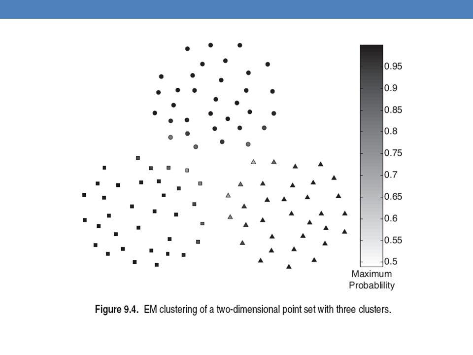
Mixture Models Once we have the parameters Θ=( 𝜋 𝐺 , 𝜋 𝐶 , 𝜇 𝐺 , 𝜇 𝐶 , 𝜎 𝐺 , 𝜎 𝐶 ) we can estimate the membership probabilities 𝑃 𝐺 𝑥 𝑖 and 𝑃 𝐶 𝑥 𝑖 for each point 𝑥 𝑖 : This is the probability that point 𝑥 𝑖 belongs to the Greek or the Chinese population (cluster) 𝑃 𝐺 𝑥 𝑖 = 𝑃 𝑥 𝑖 𝐺 𝑃(𝐺) 𝑃 𝑥 𝑖 𝐺 𝑃 𝐺 +𝑃 𝑥 𝑖 𝐶 𝑃(𝐶) = 𝑃 𝑥 𝑖 𝐺 𝜋 𝐺 𝑃 𝑥 𝑖 𝐺 𝜋 𝐺 +𝑃 𝑥 𝑖 𝐶 𝜋 𝐶
 we can estimate the membership probabilities 𝑃 𝐺 𝑥 𝑖 and 𝑃 𝐶 𝑥 𝑖 for each point 𝑥 𝑖 : This is the probability that point 𝑥 𝑖 belongs to the Greek or the Chinese population (cluster) 𝑃 𝐺 𝑥 𝑖 = 𝑃 𝑥 𝑖 𝐺 𝑃(𝐺) 𝑃 𝑥 𝑖 𝐺 𝑃 𝐺 +𝑃 𝑥 𝑖 𝐶 𝑃(𝐶) = 𝑃 𝑥 𝑖 𝐺 𝜋 𝐺 𝑃 𝑥 𝑖 𝐺 𝜋 𝐺 +𝑃 𝑥 𝑖 𝐶 𝜋 𝐶.")
26
EM (Expectation Maximization) Algorithm
Initialize the values of the parameters in Θ to some random values Repeat until convergence E-Step: Given the parameters Θ estimate the membership probabilities 𝑃 𝐺 𝑥 𝑖 and 𝑃 𝐶 𝑥 𝑖 M-Step: Compute the parameter values that (in expectation) maximize the data likelihood 𝜋 𝐺 = 1 𝑛 𝑖=1 𝑛 𝑃(𝐺| 𝑥 𝑖 ) 𝜋 𝐶 = 1 𝑛 𝑖=1 𝑛 𝑃(𝐶| 𝑥 𝑖 ) 𝜇 𝐶 = 𝑖=1 𝑛 𝑃 𝐶 𝑥 𝑖 𝑛 ∗𝜋 𝐶 𝑥 𝑖 𝜇 𝐺 = 𝑖=1 𝑛 𝑃 𝐺 𝑥 𝑖 𝑛 ∗𝜋 𝐺 𝑥 𝑖 MLE Estimates if 𝜋’s were fixed 𝜎 𝐶 2 = 𝑖=1 𝑛 𝑃 𝐶 𝑥 𝑖 𝑛 ∗𝜋 𝐶 𝑥 𝑖 − 𝜇 𝐶 2 𝜎 𝐺 2 = 𝑖=1 𝑛 𝑃 𝐺 𝑥 𝑖 𝑛 ∗𝜋 𝐺 𝑥 𝑖 − 𝜇 𝐺 2
 maximize the data likelihood. 𝜋 𝐺 = 1 𝑛 𝑖=1 𝑛 𝑃(𝐺| 𝑥 𝑖 ) 𝜋 𝐶 = 1 𝑛 𝑖=1 𝑛 𝑃(𝐶| 𝑥 𝑖 ) 𝜇 𝐶 = 𝑖=1 𝑛 𝑃 𝐶 𝑥 𝑖 𝑛 ∗𝜋 𝐶 𝑥 𝑖. 𝜇 𝐺 = 𝑖=1 𝑛 𝑃 𝐺 𝑥 𝑖 𝑛 ∗𝜋 𝐺 𝑥 𝑖. MLE Estimates. if 𝜋’s were fixed. 𝜎 𝐶 2 = 𝑖=1 𝑛 𝑃 𝐶 𝑥 𝑖 𝑛 ∗𝜋 𝐶 𝑥 𝑖 − 𝜇 𝐶 2. 𝜎 𝐺 2 = 𝑖=1 𝑛 𝑃 𝐺 𝑥 𝑖 𝑛 ∗𝜋 𝐺 𝑥 𝑖 − 𝜇 𝐺 2.")
27
Relationship to K-means
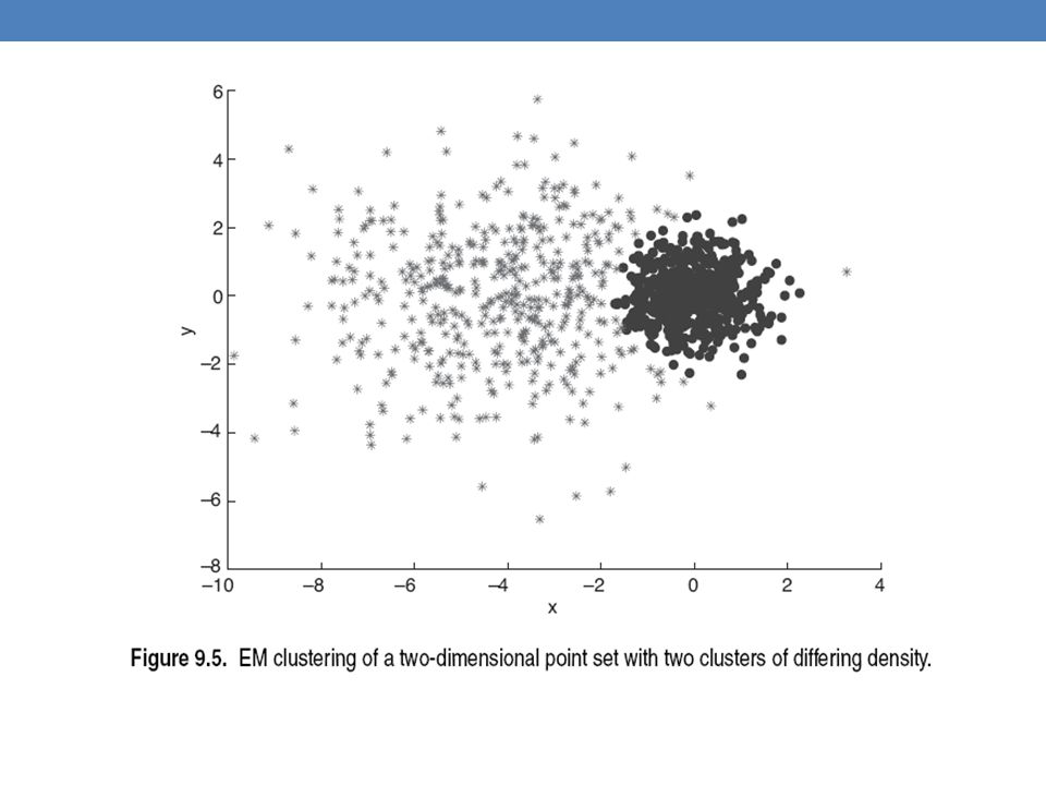
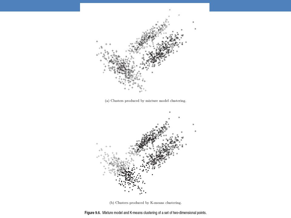
E-Step: Assignment of points to clusters K-means: hard assignment, EM: soft assignment M-Step: Computation of centroids K-means assumes common fixed variance (spherical clusters) EM: can change the variance for different clusters or different dimensions (elipsoid clusters) If the variance is fixed then both minimize the same error function
 EM: can change the variance for different clusters or different dimensions (elipsoid clusters) If the variance is fixed then both minimize the same error function.")
31
DBSCAN: A DENSITY-BASED Clustering Algorithm
Thanks to: “Introduction to Data Mining” by Tan, Steinbach, Kumar.

32
DBSCAN: Density-Based Clustering
DBSCAN is a Density-Based Clustering algorithm Reminder: In density based clustering we partition points into dense regions separated by not-so-dense regions. Important Questions: How do we measure density? What is a dense region? DBSCAN: Density at point p: number of points within a circle of radius Eps Dense Region: A circle of radius Eps that contains at least MinPts points

33
DBSCAN Characterization of points
A point is a core point if it has more than a specified number of points (MinPts) within Eps These points belong in a dense region and are at the interior of a cluster A border point has fewer than MinPts within Eps, but is in the neighborhood of a core point. A noise point is any point that is not a core point or a border point.
 within Eps. These points belong in a dense region and are at the interior of a cluster. A border point has fewer than MinPts within Eps, but is in the neighborhood of a core point. A noise point is any point that is not a core point or a border point.")
34
DBSCAN: Core, Border, and Noise Points

35
DBSCAN: Core, Border and Noise Points
Point types: core, border and noise Original Points Eps = 10, MinPts = 4

36
Density-Connected points
Density edge We place an edge between two core points q and p if they are within distance Eps. Density-connected A point p is density-connected to a point q if there is a path of edges from p to q p p1 q p q o

37
DBSCAN Algorithm Label points as core, border and noise
Eliminate noise points For every core point p that has not been assigned to a cluster Create a new cluster with the point p and all the points that are density-connected to p. Assign border points to the cluster of the closest core point.

38
DBSCAN: Determining Eps and MinPts
Idea is that for points in a cluster, their kth nearest neighbors are at roughly the same distance Noise points have the kth nearest neighbor at farther distance So, plot sorted distance of every point to its kth nearest neighbor Find the distance d where there is a “knee” in the curve Eps = d, MinPts = k Eps ~ 7-10 MinPts = 4

39
When DBSCAN Works Well Original Points Clusters Resistant to Noise
Can handle clusters of different shapes and sizes

40
When DBSCAN Does NOT Work Well
(MinPts=4, Eps=9.75). Original Points Varying densities High-dimensional data (MinPts=4, Eps=9.92)
. Original Points. Varying densities. High-dimensional data. (MinPts=4, Eps=9.92)")
41
DBSCAN: Sensitive to Parameters

42
Other algorithms PAM, CLARANS: Solutions for the k-medoids problem
BIRCH: Constructs a hierarchical tree that acts a summary of the data, and then clusters the leaves. MST: Clustering using the Minimum Spanning Tree. ROCK: clustering categorical data by neighbor and link analysis LIMBO, COOLCAT: Clustering categorical data using information theoretic tools. CURE: Hierarchical algorithm uses different representation of the cluster CHAMELEON: Hierarchical algorithm uses closeness and interconnectivity for merging

43
CLUSTERING VALIDITY

44
Cluster Validity How do we evaluate the “goodness” of the resulting clusters? But “clusters are in the eye of the beholder”! Then why do we want to evaluate them? To avoid finding patterns in noise To compare clustering algorithms To compare two sets of clusters To compare two clusters

45
Clusters found in Random Data
DBSCAN Random Points K-means Complete Link

46
Different Aspects of Cluster Validation
Determining the clustering tendency of a set of data, i.e., distinguishing whether non-random structure actually exists in the data. Comparing the results of a cluster analysis to externally known results, e.g., to externally given class labels. Evaluating how well the results of a cluster analysis fit the data without reference to external information. - Use only the data Comparing the results of two different sets of cluster analyses to determine which is better. Determining the ‘correct’ number of clusters. For 2, 3, and 4, we can further distinguish whether we want to evaluate the entire clustering or just individual clusters.

47
Measures of Cluster Validity
Numerical measures that are applied to judge various aspects of cluster validity, are classified into the following three types. External Index: Used to measure the extent to which cluster labels match externally supplied class labels. Entropy Internal Index: Used to measure the goodness of a clustering structure without respect to external information. Sum of Squared Error (SSE) Relative Index: Used to compare two different clusterings or clusters. Often an external or internal index is used for this function, e.g., SSE or entropy Sometimes these are referred to as criteria instead of indices However, sometimes criterion is the general strategy and index is the numerical measure that implements the criterion.
 Relative Index: Used to compare two different clusterings or clusters. Often an external or internal index is used for this function, e.g., SSE or entropy. Sometimes these are referred to as criteria instead of indices. However, sometimes criterion is the general strategy and index is the numerical measure that implements the criterion.")
48
Measuring Cluster Validity Via Correlation
Two matrices Proximity Matrix “Incidence” Matrix One row and one column for each data point An entry is 1 if the associated pair of points belong to the same cluster An entry is 0 if the associated pair of points belongs to different clusters Compute the correlation between the two matrices Since the matrices are symmetric, only the correlation between n(n-1) / 2 entries needs to be calculated. High correlation indicates that points that belong to the same cluster are close to each other. Not a good measure for some density or contiguity based clusters.
 / 2 entries needs to be calculated. High correlation indicates that points that belong to the same cluster are close to each other. Not a good measure for some density or contiguity based clusters.")
49
Measuring Cluster Validity Via Correlation
Correlation of incidence and proximity matrices for the K-means clusterings of the following two data sets. Corr = Corr =

50
Using Similarity Matrix for Cluster Validation
Order the similarity matrix with respect to cluster labels and inspect visually.

51
Using Similarity Matrix for Cluster Validation
Clusters in random data are not so crisp DBSCAN

52
Using Similarity Matrix for Cluster Validation
Clusters in random data are not so crisp K-means

53
Using Similarity Matrix for Cluster Validation
Clusters in random data are not so crisp Complete Link

54
Using Similarity Matrix for Cluster Validation
DBSCAN

55
Internal Measures: SSE
Clusters in more complicated figures aren’t well separated Internal Index: Used to measure the goodness of a clustering structure without respect to external information SSE SSE is good for comparing two clusterings or two clusters (average SSE). Can also be used to estimate the number of clusters
. Can also be used to estimate the number of clusters.")
56
Internal Measures: SSE
SSE curve for a more complicated data set SSE of clusters found using K-means

57
Framework for Cluster Validity
Need a framework to interpret any measure. For example, if our measure of evaluation has the value, 10, is that good, fair, or poor? Statistics provide a framework for cluster validity The more “atypical” a clustering result is, the more likely it represents valid structure in the data Can compare the values of an index that result from random data or clusterings to those of a clustering result. If the value of the index is unlikely, then the cluster results are valid These approaches are more complicated and harder to understand. For comparing the results of two different sets of cluster analyses, a framework is less necessary. However, there is the question of whether the difference between two index values is significant

58
Statistical Framework for SSE
Example Compare SSE of against three clusters in random data Histogram shows SSE of three clusters in 500 sets of random data points of size 100 distributed over the range 0.2 – 0.8 for x and y values

59
Statistical Framework for Correlation
Correlation of incidence and proximity matrices for the K-means clusterings of the following two data sets. Corr = Corr =

60
Internal Measures: Cohesion and Separation
Cluster Cohesion: Measures how closely related are objects in a cluster Example: SSE Cluster Separation: Measure how distinct or well-separated a cluster is from other clusters Example: Squared Error Cohesion is measured by the within cluster sum of squares (SSE) Separation is measured by the between cluster sum of squares Where |Ci| is the size of cluster i
 Separation is measured by the between cluster sum of squares. Where |Ci| is the size of cluster i.")
61
Internal Measures: Cohesion and Separation
A proximity graph based approach can also be used for cohesion and separation. Cluster cohesion is the sum of the weight of all links within a cluster. Cluster separation is the sum of the weights between nodes in the cluster and nodes outside the cluster. cohesion separation

62
External Measures for Clustering Validity
Assume that the data is labeled with some class labels E.g., documents are classified into topics, people classified according to their income, senators classified as republican or democrat. In this case we want the clusters to be homogeneous with respect to classes Each cluster should contain elements of mostly one class Also each class should ideally be assigned to a single cluster This does not always make sense Clustering is not the same as classification But this is what people use most of the time

63
Measures 𝑚 = number of points 𝑚 𝑖 = points in cluster i
𝑚 𝑗 = points in class j 𝑚 𝑖𝑗 = points in cluster i coming from class j 𝑝 𝑖𝑗 = 𝑚 𝑖𝑗 / 𝑚 𝑖 = prob of element from class j in cluster i Entropy: Of a cluster i: 𝑒 𝑖 =− 𝑗=1 𝐿 𝑝 𝑖𝑗 log 𝑝 𝑖𝑗 Highest when uniform, zero when single class Of a clustering: 𝑒= 𝑖=1 𝐾 𝑚 𝑖 𝑚 𝑒 𝑖 Purity: Of a cluster i: 𝑝 𝑖 = max 𝑗 𝑝 𝑖𝑗 Of a clustering: 𝑝𝑢𝑟𝑖𝑡𝑦= 𝑖=1 𝐾 𝑚 𝑖 𝑚 𝑝 𝑖

64
Measures Precision: Recall: F-measure:
Of cluster i with respect to class j: 𝑃𝑟𝑒𝑐 𝑖,𝑗 = 𝑝 𝑖𝑗 Recall: Of cluster I with respect to class j: 𝑅𝑒𝑐 𝑖,𝑗 = 𝑚 𝑖𝑗 𝑚 𝑗 F-measure: Harmonic Mean of Precision and Recall: 𝐹 𝑖,𝑗 = 2∗𝑃𝑟𝑒𝑐 𝑖,𝑗 ∗𝑅𝑒𝑐(𝑖,𝑗) 𝑃𝑟𝑒𝑐 𝑖,𝑗 +𝑅𝑒𝑐(𝑖,𝑗)
 𝑃𝑟𝑒𝑐 𝑖,𝑗 +𝑅𝑒𝑐(𝑖,𝑗)")
65
External Measures of Cluster Validity: Entropy and Purity

66
Final Comment on Cluster Validity
“The validation of clustering structures is the most difficult and frustrating part of cluster analysis. Without a strong effort in this direction, cluster analysis will remain a black art accessible only to those true believers who have experience and great courage.” Algorithms for Clustering Data, Jain and Dubes

Παρόμοιες παρουσιάσεις